Get certified for free when you join Fabric Data Days 2026 and dive into Fabric, Power BI, SQL, AI, and other essential data skills.
Join nowJuly 7 - July 17 | Round 2 of the Power BI Dataviz World Championships. Don't miss your chance! Learn more
Can somebody help me with the Power Query code by which I can update the value for Column Spend for against ProductTitle Diff whose formula is Base = 1 – SUM(Spend). Data may increase and pattern is shown below. The source is SharePoint list. I will have to show this data on Donut chart in Power BI.
Spend ReportDate ProductTitle Spend ReportDate ProductTitle
0.3 5/4/2016 A 0.3 5/4/2016 A
0.53 5/4/2016 B 0.53 5/4/2016 B
5/4/2016 Base 0.17 5/4/2016 Base
Spend ReportDate ProductTitle Spend ReportDate ProductTitle
0.3 5/4/2016 A 0.3 5/4/2016 A
0.53 5/4/2016 B 0.53 5/4/2016 B
5/4/2016 Base 0.17 5/4/2016 Base
0.5 6/5/2016 A 0.5 6/5/2016 A
0.38 6/5/2016 B 0.38 6/5/2016 B
6/5/2016 Base 0.12 6/5/2016 Base
Solved! Go to Solution.
Here are the detailed steps for achieving this. I am asuming that your Product title has same pattren.
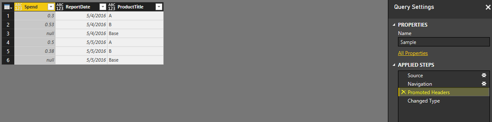
I have used below sample data in excel
Connected with Excel and edit the query
After this remove the two steps from right area "Chagne Type" and Promoted Headers". It will bring your column hearders as data row. Now remove first row by going to Home Table and clicking Remove Rows button. You need to mention 1 as number of rows to be deleted.
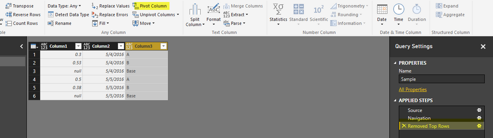
Now your data set will look like this.
Now select Column3 and click on Pivot Column button under Transformations Tab
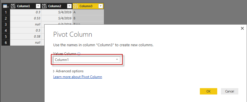
select Column1 as Value column in popup and click Ok. It will pivot your data to a new format as below
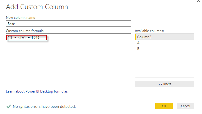
Now remove the Base Column and Add new Column Base with Below Formula
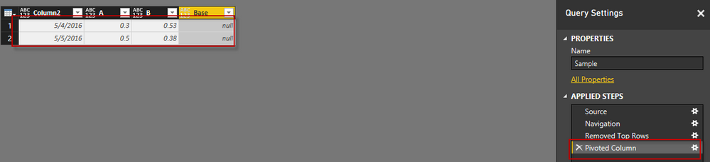
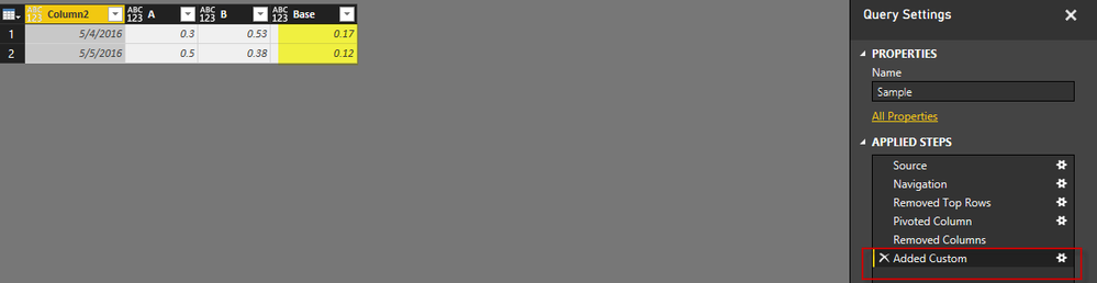
You base value has been calculated. See below for reference
Here are the detailed steps for achieving this. I am asuming that your Product title has same pattren.
I have used below sample data in excel
Connected with Excel and edit the query
After this remove the two steps from right area "Chagne Type" and Promoted Headers". It will bring your column hearders as data row. Now remove first row by going to Home Table and clicking Remove Rows button. You need to mention 1 as number of rows to be deleted.
Now your data set will look like this.
Now select Column3 and click on Pivot Column button under Transformations Tab
select Column1 as Value column in popup and click Ok. It will pivot your data to a new format as below
Now remove the Base Column and Add new Column Base with Below Formula
You base value has been calculated. See below for reference
Thank You so much Habib for your time and support. This solution has helped me to complete my task. Thanks again...![]()
Join us in Barcelona for FabCon and SQLCon, the Fabric, Power BI, SQL, and AI community event. Save €200 with code FABCMTY200.
Join Data Days 2026: 60 days of free live/on-demand sessions, challenges, study groups, and certification opportunities.
| User | Count |
|---|---|
| 24 | |
| 10 | |
| 10 | |
| 6 | |
| 4 |
| User | Count |
|---|---|
| 32 | |
| 25 | |
| 18 | |
| 18 | |
| 17 |