- Power BI forums
- Get Help with Power BI
- Desktop
- Service
- Report Server
- Power Query
- Mobile Apps
- Developer
- DAX Commands and Tips
- Custom Visuals Development Discussion
- Health and Life Sciences
- Power BI Spanish forums
- Translated Spanish Desktop
- Training and Consulting
- Instructor Led Training
- Dashboard in a Day for Women, by Women
- Galleries
- Data Stories Gallery
- Themes Gallery
- Contests Gallery
- QuickViz Gallery
- Quick Measures Gallery
- Visual Calculations Gallery
- Notebook Gallery
- Translytical Task Flow Gallery
- TMDL Gallery
- R Script Showcase
- Webinars and Video Gallery
- Ideas
- Custom Visuals Ideas (read-only)
- Issues
- Issues
- Events
- Upcoming Events
Learn from the best! Meet the four finalists headed to the FINALS of the Power BI Dataviz World Championships! Register now
- Power BI forums
- Forums
- Get Help with Power BI
- Power Query
- Compare two cells value
- Subscribe to RSS Feed
- Mark Topic as New
- Mark Topic as Read
- Float this Topic for Current User
- Bookmark
- Subscribe
- Printer Friendly Page
- Mark as New
- Bookmark
- Subscribe
- Mute
- Subscribe to RSS Feed
- Permalink
- Report Inappropriate Content
Compare two cells value
Hi there,
my need is to color 2 cells of the same column if they have the same value; for example:
| REF | COLORTHAT |
| ABC | THISYES |
| DEF | THISNO |
| GHI | THISYES |
thanks
Solved! Go to Solution.
- Mark as New
- Bookmark
- Subscribe
- Mute
- Subscribe to RSS Feed
- Permalink
- Report Inappropriate Content
Hi @Mikahel369 ,
According to your description, here's my solution.
Create a measure.
Color =
IF (
    COUNTROWS (
        FILTER ( ALL ( 'Table' ), 'Table'[COLORTHAT] = MAX ( 'Table'[COLORTHAT] ) )
    ) > 1,
    "Red"
)
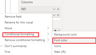
In the visualizations pane, select the drop-box of COLORTHAT, then click Conditional formatting>Font color.
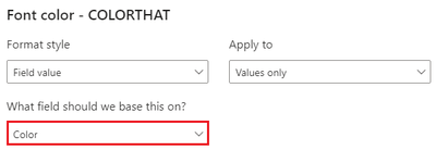
Select the measure in the dialog.
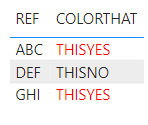
Get the expected result:
I attach my sample below for your reference.
Best Regards,
Community Support Team _ kalyj
If this post helps, then please consider Accept it as the solution to help the other members find it more quickly.
- Mark as New
- Bookmark
- Subscribe
- Mute
- Subscribe to RSS Feed
- Permalink
- Report Inappropriate Content
You can use this formula in conditional fomatting.
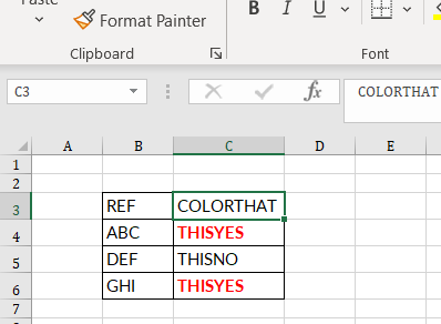
Select first the range in which you want to apply the conditional formatting (in my case C3:C6)
Go to the HOME --> Conditional formatting --> New rules --> "Use formula ..:".
Paste this formula to the box--> =IF(COUNTIF($C$3:$C$6;C3)>1;TRUE;FALSE)
Click FORMAT and adjust the formatting and then press OK.
If it doesn't work get back and remove from the formula the double quotes.
✅ Check the question as solved if I helped you.
You can follow me on LinkedIn:
- Mark as New
- Bookmark
- Subscribe
- Mute
- Subscribe to RSS Feed
- Permalink
- Report Inappropriate Content
Hi @Mikahel369 ,
According to your description, here's my solution.
Create a measure.
Color =
IF (
    COUNTROWS (
        FILTER ( ALL ( 'Table' ), 'Table'[COLORTHAT] = MAX ( 'Table'[COLORTHAT] ) )
    ) > 1,
    "Red"
)
In the visualizations pane, select the drop-box of COLORTHAT, then click Conditional formatting>Font color.
Select the measure in the dialog.
Get the expected result:
I attach my sample below for your reference.
Best Regards,
Community Support Team _ kalyj
If this post helps, then please consider Accept it as the solution to help the other members find it more quickly.
- Mark as New
- Bookmark
- Subscribe
- Mute
- Subscribe to RSS Feed
- Permalink
- Report Inappropriate Content
- Mark as New
- Bookmark
- Subscribe
- Mute
- Subscribe to RSS Feed
- Permalink
- Report Inappropriate Content
I'll move elsewhere... if I found how to
Helpful resources
| User | Count |
|---|---|
| 5 | |
| 4 | |
| 3 | |
| 3 | |
| 3 |
| User | Count |
|---|---|
| 13 | |
| 8 | |
| 8 | |
| 7 | |
| 6 |


