cancel
Showing results for 
Search instead for 
Did you mean: 

The Fabric community is upgrading! Read all of the details including the timeline and what you can expect. Learn more

Reply
Mikahel369
Frequent Visitor

Compare two cells value

Hi there,


my need is to color 2 cells of the same column if they have the same value; for example:


REFCOLORTHAT
ABCTHISYES
DEF

THISNO

GHITHISYES


thanks

1 ACCEPTED SOLUTION
v-yanjiang-msft
Community Support
Community Support

Hi @Mikahel369 ,

According to your description, here's my solution.

Create a measure.

Color =
IF (
    COUNTROWS (
        FILTER ( ALL ( 'Table' ), 'Table'[COLORTHAT] = MAX ( 'Table'[COLORTHAT] ) )
    ) > 1,
    "Red"
)

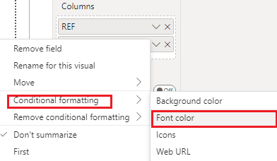
In the visualizations pane, select the drop-box of COLORTHAT, then click Conditional formatting>Font color.

vkalyjmsft_0-1667462151849.png

vkalyjmsft_1-1667462200739.png

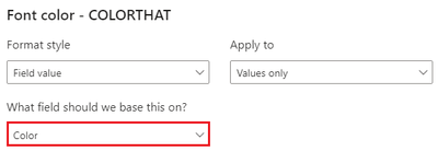
Select the measure in the dialog.

vkalyjmsft_3-1667462346648.png

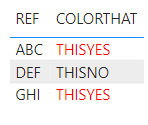
Get the expected result:

vkalyjmsft_4-1667462380797.png

I attach my sample below for your reference.


Best Regards,
Community Support Team _ kalyj

If this post helps, then please consider Accept it as the solution to help the other members find it more quickly.


View solution in original post

4 REPLIES 4
AKNiang
Frequent Visitor


You can use this formula in conditional fomatting.


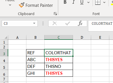
Select first the range in which you want to apply the conditional formatting (in my case C3:C6)


AKNiang_0-1667467657823.png


Go to the HOME --> Conditional formatting --> New rules --> "Use formula ..:".


Paste this formula to the box--> =IF(COUNTIF($C$3:$C$6;C3)>1;TRUE;FALSE)


Click FORMAT and adjust the formatting and then press OK.


If it doesn't work get back and remove from the formula the double quotes.


Check the question as solved if I helped you. 

You can follow me on LinkedIn:

(1) Abdoul Karim Niang | LinkedIn

v-yanjiang-msft
Community Support
Community Support

Hi @Mikahel369 ,

According to your description, here's my solution.

Create a measure.

Color =
IF (
    COUNTROWS (
        FILTER ( ALL ( 'Table' ), 'Table'[COLORTHAT] = MAX ( 'Table'[COLORTHAT] ) )
    ) > 1,
    "Red"
)

In the visualizations pane, select the drop-box of COLORTHAT, then click Conditional formatting>Font color.

vkalyjmsft_0-1667462151849.png

vkalyjmsft_1-1667462200739.png

Select the measure in the dialog.

vkalyjmsft_3-1667462346648.png

Get the expected result:

vkalyjmsft_4-1667462380797.png

I attach my sample below for your reference.


Best Regards,
Community Support Team _ kalyj

If this post helps, then please consider Accept it as the solution to help the other members find it more quickly.


AntrikshSharma
Community Champion
Community Champion

@Mikahel369 Coloring cells is not possible in Power Query.

I'll move elsewhere... if I found how to

Helpful resources

Announcements
FabCon and SQLCon Barcelona 2026

FabCon & SQLCon – Barcelona 2026

Join us in Barcelona for FabCon and SQLCon, the Fabric, Power BI, SQL, and AI community event. Save €200 with code FABCMTY200.

Power BI DataViz World Championships carousel

Power BI DataViz World Championships - June 2026

A new Power BI DataViz World Championship is coming this June! Don't miss out on submitting your entry.