cancel
Showing results for 
Search instead for 
Did you mean: 

July 28 - August 9 | Final Round of the Power BI Dataviz World Championships. This is your chance. Learn more

Reply
Mikahel369
Frequent Visitor

Compare two cells value

Hi there,


my need is to color 2 cells of the same column if they have the same value; for example:


REFCOLORTHAT
ABCTHISYES
DEF

THISNO

GHITHISYES


thanks

1 ACCEPTED SOLUTION
v-yanjiang-msft
Community Support
Community Support

Hi @Mikahel369 ,

According to your description, here's my solution.

Create a measure.

Color =
IF (
    COUNTROWS (
        FILTER ( ALL ( 'Table' ), 'Table'[COLORTHAT] = MAX ( 'Table'[COLORTHAT] ) )
    ) > 1,
    "Red"
)

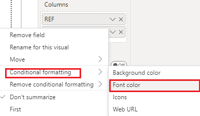
In the visualizations pane, select the drop-box of COLORTHAT, then click Conditional formatting>Font color.

vkalyjmsft_0-1667462151849.png

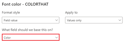
vkalyjmsft_1-1667462200739.png

Select the measure in the dialog.

vkalyjmsft_3-1667462346648.png

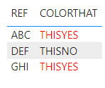
Get the expected result:

vkalyjmsft_4-1667462380797.png

I attach my sample below for your reference.


Best Regards,
Community Support Team _ kalyj

If this post helps, then please consider Accept it as the solution to help the other members find it more quickly.


View solution in original post

4 REPLIES 4
AKNiang
Frequent Visitor


You can use this formula in conditional fomatting.


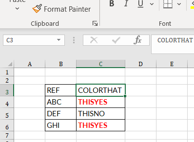
Select first the range in which you want to apply the conditional formatting (in my case C3:C6)


AKNiang_0-1667467657823.png


Go to the HOME --> Conditional formatting --> New rules --> "Use formula ..:".


Paste this formula to the box--> =IF(COUNTIF($C$3:$C$6;C3)>1;TRUE;FALSE)


Click FORMAT and adjust the formatting and then press OK.


If it doesn't work get back and remove from the formula the double quotes.


Check the question as solved if I helped you. 

You can follow me on LinkedIn:

(1) Abdoul Karim Niang | LinkedIn

v-yanjiang-msft
Community Support
Community Support

Hi @Mikahel369 ,

According to your description, here's my solution.

Create a measure.

Color =
IF (
    COUNTROWS (
        FILTER ( ALL ( 'Table' ), 'Table'[COLORTHAT] = MAX ( 'Table'[COLORTHAT] ) )
    ) > 1,
    "Red"
)

In the visualizations pane, select the drop-box of COLORTHAT, then click Conditional formatting>Font color.

vkalyjmsft_0-1667462151849.png

vkalyjmsft_1-1667462200739.png

Select the measure in the dialog.

vkalyjmsft_3-1667462346648.png

Get the expected result:

vkalyjmsft_4-1667462380797.png

I attach my sample below for your reference.


Best Regards,
Community Support Team _ kalyj

If this post helps, then please consider Accept it as the solution to help the other members find it more quickly.


AntrikshSharma
Community Champion
Community Champion

@Mikahel369 Coloring cells is not possible in Power Query.

I'll move elsewhere... if I found how to

Helpful resources

Announcements
Fabric Community Sticker Design Challenge Barcelona Carousel

Fabric Community Sticker Challenge - Barcelona 2026

If you love stickers, then you will definitely want to check out our community sticker challenge, Barcelona edition!

July Power BI Update Carousel

Power BI Monthly Update - July 2026

Check out the July 2026 Power BI update to learn about new features.

Power BI DataViz World Championships carousel

Power BI DataViz World Championships - June 2026

A new Power BI DataViz World Championship is coming this June! Don't miss out on submitting your entry.