FabCon is coming to Atlanta
Join us at FabCon Atlanta from March 16 - 20, 2026, for the ultimate Fabric, Power BI, AI and SQL community-led event. Save $200 with code FABCOMM.
Register now!- Power BI forums
- Get Help with Power BI
- Desktop
- Service
- Report Server
- Power Query
- Mobile Apps
- Developer
- DAX Commands and Tips
- Custom Visuals Development Discussion
- Health and Life Sciences
- Power BI Spanish forums
- Translated Spanish Desktop
- Training and Consulting
- Instructor Led Training
- Dashboard in a Day for Women, by Women
- Galleries
- Data Stories Gallery
- Themes Gallery
- Contests Gallery
- QuickViz Gallery
- Quick Measures Gallery
- Visual Calculations Gallery
- Notebook Gallery
- Translytical Task Flow Gallery
- TMDL Gallery
- R Script Showcase
- Webinars and Video Gallery
- Ideas
- Custom Visuals Ideas (read-only)
- Issues
- Issues
- Events
- Upcoming Events
The Power BI Data Visualization World Championships is back! Get ahead of the game and start preparing now! Learn more
- Power BI forums
- Forums
- Get Help with Power BI
- Desktop
- Re: VAR formula with multiple return values
- Subscribe to RSS Feed
- Mark Topic as New
- Mark Topic as Read
- Float this Topic for Current User
- Bookmark
- Subscribe
- Printer Friendly Page
- Mark as New
- Bookmark
- Subscribe
- Mute
- Subscribe to RSS Feed
- Permalink
- Report Inappropriate Content
VAR formula with multiple return values
Hi,
I have data set with week1 , week2, week3, week4 and with the staus of "Completed", "inprogress" and "Failed".
I used below formul to do the conditional formatting in my data set since it has text values.
This formulas is only works for "Completed". I want to created this formulas to highlight "Inprogress and "Failed" status as well.
Also I want to apply this same formul to week2,3,4 as well.
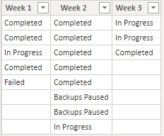
When I add this formula to week 2 it will hight the same values in week 1. Please check the attached picture.
Can anyone help me to do this
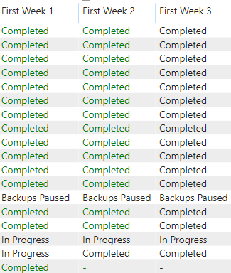
Solved! Go to Solution.
- Mark as New
- Bookmark
- Subscribe
- Mute
- Subscribe to RSS Feed
- Permalink
- Report Inappropriate Content
Hi,
According to your description, I create a simple sample to test:
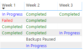
The issue is because that you apply one measure to all columns.
So for each row, it will show the same color regardless of the value, like this:
color =
var w1 = SELECTEDVALUE('Table'[Week 1])
var w2 = SELECTEDVALUE('Table'[Week 2])
var w3 = SELECTEDVALUE('Table'[Week 3])
return
SWITCH(true,w1="Completed","Green",w1="In Progress","Blue",w1="Failed","Red",
            w2="Completed","Green",w2="In Progress","Blue",w2="Failed","Red",
            w3="Completed","Green",w3="In Progress","Blue",w3="Failed","Red"
)
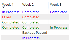
Please try to create measures for each week:
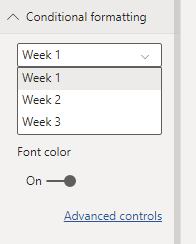
Measure 1 = SWITCH(SELECTEDVALUE('Table'[Week 1]),"Completed","Green","In Progress","Blue","Failed","Red")Measure 2 = SWITCH(SELECTEDVALUE('Table'[Week 2]),"Completed","Green","In Progress","Blue","Failed","Red")Measure 3 = SWITCH(SELECTEDVALUE('Table'[Week 3]),"Completed","Green","In Progress","Blue","Failed","Red")Then apply these to each week's font color:
And the result shows:
Hope this helps.
Best Regards,
Giotto Zhi
- Mark as New
- Bookmark
- Subscribe
- Mute
- Subscribe to RSS Feed
- Permalink
- Report Inappropriate Content
- Mark as New
- Bookmark
- Subscribe
- Mute
- Subscribe to RSS Feed
- Permalink
- Report Inappropriate Content
Hi,
If you want to add conditionnal formating within a table or matrix, I would recommend to use the conditionnal formating option in th e vizualization panel.
Please see the below article :
https://docs.microsoft.com/en-us/power-bi/desktop-conditional-table-formatting
Hope it will help 🙂
- Mark as New
- Bookmark
- Subscribe
- Mute
- Subscribe to RSS Feed
- Permalink
- Report Inappropriate Content
Hi @Anonymous ,
Since I have text values in my data set I cannot use conditional formatting. I already treid that. That's why I used this formula. Can you help me with this formula. Or any other way?
- Mark as New
- Bookmark
- Subscribe
- Mute
- Subscribe to RSS Feed
- Permalink
- Report Inappropriate Content
Hi,
Can you share the pbix file with me ?
I think you should create a new table with the status + ID (Number) and used the ID to do the conditionnal formating.
But I need to see how did you build your data model.
Thanks
Helpful resources

Power BI Dataviz World Championships
The Power BI Data Visualization World Championships is back! Get ahead of the game and start preparing now!

| User | Count |
|---|---|
| 40 | |
| 35 | |
| 34 | |
| 31 | |
| 28 |
| User | Count |
|---|---|
| 136 | |
| 102 | |
| 68 | |
| 66 | |
| 58 |
