A new Data Days event is coming soon!
This time we’re going bigger than ever. Fabric, Power BI, SQL, AI and more. We're covering it all. You won't want to miss it.
Learn more- Power BI forums
- Get Help with Power BI
- Desktop
- Service
- Report Server
- Power Query
- Mobile Apps
- Developer
- DAX Commands and Tips
- Custom Visuals Development Discussion
- Health and Life Sciences
- Power BI Spanish forums
- Translated Spanish Desktop
- Training and Consulting
- Instructor Led Training
- Dashboard in a Day for Women, by Women
- Galleries
- Data Stories Gallery
- Themes Gallery
- Contests Gallery
- QuickViz Gallery
- Quick Measures Gallery
- Visual Calculations Gallery
- Notebook Gallery
- Translytical Task Flow Gallery
- TMDL Gallery
- R Script Showcase
- Webinars and Video Gallery
- Ideas
- Custom Visuals Ideas (read-only)
- Issues
- Issues
- Events
- Upcoming Events
Level up your Power BI skills this month - build one visual each week and tell better stories with data! Get started
- Power BI forums
- Galleries
- R Script Showcase
- Re: R multiple visual in one: Regression Table and...
Your file has been submitted successfully. We’re processing it now - please check back in a few minutes to view your report.
Re: R multiple visual in one: Regression Table and Boxplot
07-15-2024 09:00 AM - last edited 07-15-2024 09:32 AM
- Mark as New
- Bookmark
- Subscribe
- Mute
- Subscribe to RSS Feed
- Permalink
- Report Inappropriate Content
R multiple visual in one: Regression Table and Boxplot
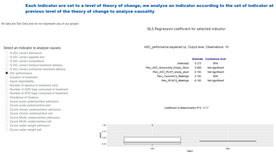
In this pbix File, we construct an analysis of Theory of change and create a R visual that gather a regression analysis and a Boxplot visual.
Theory of change is a theoritical relation between indicators:
Gestion -> Output -> Outcome -> Impact
How we do -> What we do -> Why we do -> General Objective
- Mark as New
- Bookmark
- Subscribe
- Mute
- Subscribe to RSS Feed
- Permalink
- Report Inappropriate Content
UPDATE 02/2025:
- Mark as New
- Bookmark
- Subscribe
- Mute
- Subscribe to RSS Feed
- Permalink
- Report Inappropriate Content
UPDATE 'base2grob' is no longer available
Here is an adapted version with ggplot2.
I've also performed a t-test that check whether there is sufficient observations or not.
Here is the visual code:


