Fabric Data Days starts November 4th!
Advance your Data & AI career with 50 days of live learning, dataviz contests, hands-on challenges, study groups & certifications and more!
Get registered- Power BI forums
- Get Help with Power BI
- Desktop
- Service
- Report Server
- Power Query
- Mobile Apps
- Developer
- DAX Commands and Tips
- Custom Visuals Development Discussion
- Health and Life Sciences
- Power BI Spanish forums
- Translated Spanish Desktop
- Training and Consulting
- Instructor Led Training
- Dashboard in a Day for Women, by Women
- Galleries
- Data Stories Gallery
- Themes Gallery
- Contests Gallery
- QuickViz Gallery
- Quick Measures Gallery
- Visual Calculations Gallery
- Notebook Gallery
- Translytical Task Flow Gallery
- TMDL Gallery
- R Script Showcase
- Webinars and Video Gallery
- Ideas
- Custom Visuals Ideas (read-only)
- Issues
- Issues
- Events
- Upcoming Events
Get Fabric Certified for FREE during Fabric Data Days. Don't miss your chance! Request now
- Power BI forums
- Forums
- Get Help with Power BI
- Desktop
- Filter out unique values from the cell that contai...
- Subscribe to RSS Feed
- Mark Topic as New
- Mark Topic as Read
- Float this Topic for Current User
- Bookmark
- Subscribe
- Printer Friendly Page
- Mark as New
- Bookmark
- Subscribe
- Mute
- Subscribe to RSS Feed
- Permalink
- Report Inappropriate Content
Filter out unique values from the cell that contains multiple values
Hi,
I have a column that contains multiple values and I want to create a new column that keeps the unique values only from the original one.
Example:
- if the multiple value is "Springfield, Springfield, Pueblo West", the new column should show "Springfield, Pueblo West".
- if the multiple value is "Springfield, Springfield, Springfield", the new column should show "Springfield".
Is there a way to create a calculated column that solves this?
This is the mage of the column and wanted result in red colour.
Best,
Solved! Go to Solution.
- Mark as New
- Bookmark
- Subscribe
- Mute
- Subscribe to RSS Feed
- Permalink
- Report Inappropriate Content
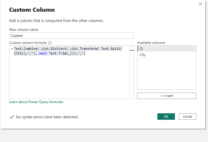
You can solve this by adding a custom column in Power Query. On the "Add Column" tab click on Custom Coulmn option and type the next code :
Text.Combine( List.Distinct( List.Transform( Text.Split([City],","), each Text.Trim(_))),",")
The result will be unique values separated by comma in each cell.
Best
- Mark as New
- Bookmark
- Subscribe
- Mute
- Subscribe to RSS Feed
- Permalink
- Report Inappropriate Content
Hi,
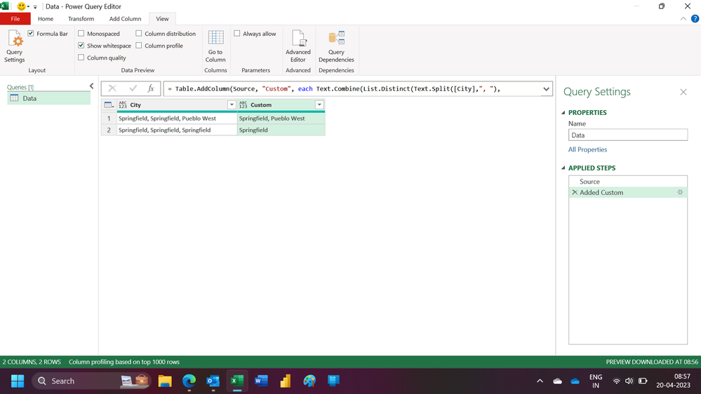
This M code works
let
    Source = Excel.CurrentWorkbook(){[Name="Data"]}[Content],
    #"Added Custom" = Table.AddColumn(Source, "Custom", each Text.Combine(List.Distinct(Text.Split([City],", "),Comparer.OrdinalIgnoreCase),", "))
in
    #"Added Custom"
Hope this helps.
Regards,
Ashish Mathur
http://www.ashishmathur.com
https://www.linkedin.com/in/excelenthusiasts/
- Mark as New
- Bookmark
- Subscribe
- Mute
- Subscribe to RSS Feed
- Permalink
- Report Inappropriate Content
Hi @arinyc ,
Here are the steps you can follow:
1. In Power Query -- Add Column – Index Column – From 1.
2. Copy Table to Table2.
3. Select [City] – Transform – Split column:
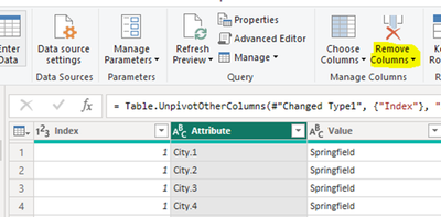
4. Select [City.1] – [City.6] – Transform – Unpivot Columns.

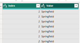
6. Select the two columns – Right click – Remove Duplications.
Result:
7. Create calculated column.
Column =
CONCATENATEX(
    FILTER(ALL('Table2'),
    'Table2'[Index]=EARLIER('Table'[Index])),[Value],",")
8. Result:
Best Regards,
Liu Yang
If this post helps, then please consider Accept it as the solution to help the other members find it more quickly
- Mark as New
- Bookmark
- Subscribe
- Mute
- Subscribe to RSS Feed
- Permalink
- Report Inappropriate Content
In addition to my original post and question here is a GDrive LINK with sample data in PBI format.
Helpful resources

Power BI Monthly Update - November 2025
Check out the November 2025 Power BI update to learn about new features.

Fabric Data Days
Advance your Data & AI career with 50 days of live learning, contests, hands-on challenges, study groups & certifications and more!

| User | Count |
|---|---|
| 97 | |
| 73 | |
| 50 | |
| 47 | |
| 44 |


