DAX match text in multiple columns

[AshleyMartinez]

Hi,

I've been trying to figure out how can I get this report done but I can't find any efficient way to fo it.

I have 2 tables:

[Table1] Sales by brand and date:

Brand	Date	Sales
Apple	Jan-19	2.30
Huawei	Jan-19	2.18
Lenovo	Jan-19	0.80
LG	Jan-19	1.10
Samsung	Jan-19	1.90
Xiaomi	Jan-19	1.70
Apple	Feb-19	2.40
Huawei	Feb-19	2.15
Lenovo	Feb-19	0.60
LG	Feb-19	1.20
Samsung	Feb-19	1.80
Xiaomi	Feb-19	1.60

[Table2] And all the workers responsible (in any way) for each brand. Every worker can have different positions by brand, they can even have more than one position by brand.

Brand	City Agent	Region Agent	Country Agent	Head of Account
Apple	Mike	Carl	Mike	Bryan
Huawei	Jane	Florence	Jane	Bryan
Samsung	Mike	Lucia	Bryan	Bryan
Xiaomi	Carl	Jane	Bryan	Florence
LG	Carl	Florence	Lucia	Lucia
Lenovo	Mike	Mike	Jane	Florence

What I need is to get sales by worker.

The logic is: If I want see Bryan, the formula should look if Bryan is in any of the four columns (city agent, region agent, country agent, head of  account) at least once in [Table2], if so, then bring the sales corresponding to every brand in which Bryan has had a match, like this:

Worker	Brand	Jan-19	Feb-19
Bryan	Apple	2.3	2.4
Bryan	Huawei	2.18	2.15
Bryan	Samsung	1.9	1.8
Bryan	Xiaomi	1.7	1.6
Total		8.08	7.95

*See that Bryan has 2 positions in Samsung (Country Agent and Head of Account) but the sales are not duplicated and that's correct.

Obviously, if I see all the workers in one table, the sales are going to be repeated as many times as different workers asigned to each brand, and that's ok, like this:

Worker	Jan-19	Feb-19	Total
Bryan	8.08	7.95	16.03
Carl	5.1	5.2	10.3
Florence	5.78	5.55	11.33
Jane	4.68	4.35	9.03
Lucia	3	3	6
Mike	5	4.8	9.8
Total	31.64	30.85	62.49

I've created tables to relate [Table1] and [Table2] without success.

Any ideas? PLEASE!

[AshleyMartinez]

The new sales table would be like this:

Brand	Date	Sales
Apple	Jan-19	2.3
Apple	Jan-19	0.4
Huawei	Jan-19	2.18
Lenovo	Jan-19	0.8
LG	Jan-19	1.1
Samsung	Jan-19	1.9
Samsung	Jan-19	1.3
Xiaomi	Jan-19	1.7
Apple	Feb-19	2.4
Huawei	Feb-19	2.15
Lenovo	Feb-19	0.6
Lenovo	Feb-19	0.2
LG	Feb-19	1.2
Samsung	Feb-19	1.8
Xiaomi	Feb-19	1.6

[Nathaniel_C]

Hi @AshleyMartinez , @smpa01 ,

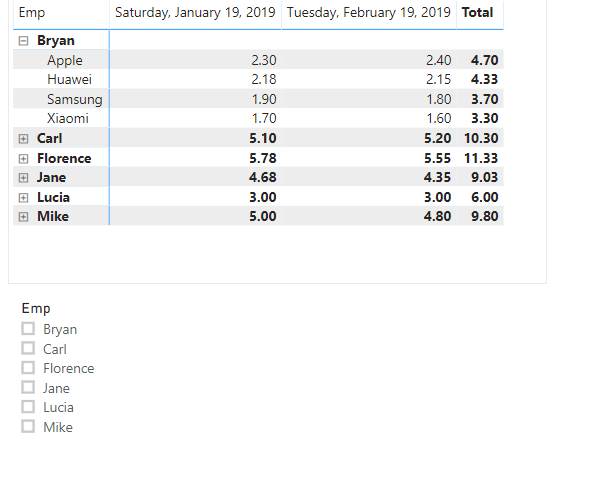
I believe this is the output for which you were looking... created the table that I show in the picture. Automated in PQ. Then did a join between the two tables.  It is many to many, so you might want to consider an intermediate table, but it works.  Here is the pbix. My pbix 

I had to recreate this as I went down another road trying to set your data in a normal fashion. Exploring a table for each classification of agent would be for starters.  I find if one uses a star schema from the beginning things work better down the road. You may have this, and we are only seeing a couple of tables.

How ever, I was able to rebuild it from what I had posted here.  Anyway this seems to meet your requirements. Please let me know if you have any questions.

If this solves your issues, please mark it as the solution, so that others can find it easily. Kudos are nice too.
Nathaniel

[AshleyMartinez]

Hi! @smpa01 

I'm working on your approach, and it's working flawless with the example. Now, applying this to my actual data, I have a problem and is that I have more than one row of sales per day for the same brand, which means that the measure added ("Sales") in NewTbl has to sum sales grouped by "Name", "Brand", "Date". I've been trying Summarize but the error is: "the expression refers to multiple columns.."

@Nathaniel_C 

I unpivot Table 2 but I don't know why I can't get the same results as you, can you share your file?

Thank you so much for your time!

[smpa01]

@AshleyMartinez  can you please try this.

NewTbl = 
VAR _x = SELECTCOLUMNS (
    'Table 2',
    "Name", 'Table 2'[City Agent],
    "Brand", 'Table 2'[Brand]&""
)
VAR _y = SELECTCOLUMNS (
    'Table 2',
    "Name", 'Table 2'[Country Agent],
    "Brand", 'Table 2'[Brand]&""
)
VAR _z = SELECTCOLUMNS (
    'Table 2',
    "Name", 'Table 2'[Head of Account],
    "Brand", 'Table 2'[Brand]&""
)
VAR _a= SELECTCOLUMNS (
    'Table 2',
    "Name", 'Table 2'[Region Agent],
    "Brand", 'Table 2'[Brand]&""
)
 VAR _t= DISTINCT
                 (
                   UNION(_x,_y,_z,_a)
                 )
VAR _d= DISTINCT(SELECTCOLUMNS('Table 5',"Date",'Table 5'[Date]))
VAR _cross = CROSSJOIN(_t,_d)
VAR _new = SELECTCOLUMNS(
    'Table 5',
    "Brand",'Table 5'[Brand]&"",
    "Date",'Table 5'[Date],
    "Sales",'Table 5'[Sales]
)
VAR _sz = NATURALLEFTOUTERJOIN(_cross,_new)
RETURN _sz

[Nathaniel_C]

Hi @AshleyMartinez , @smpa01 ,

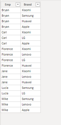
Automated change in PQ.

let
    Source = Excel.Workbook(File.Contents("C:\Users\nat_c\OneDrive\Desktop\SalesBrand.xlsx"), null, true),
    Brand_Table = Source{[Item="Brand",Kind="Table"]}[Data],
    #"Changed Type" = Table.TransformColumnTypes(Brand_Table,{{"Brand", type text}, {"City Agent", type text}, {"Region Agent", type text}, {"Country Agent", type text}, {"Head of Account", type text}}),
    #"Unpivoted Columns" = Table.UnpivotOtherColumns(#"Changed Type", {"Brand"}, "Attribute", "Value"),
    #"Removed Columns" = Table.RemoveColumns(#"Unpivoted Columns",{"Attribute"}),
    #"Merged Columns" = Table.CombineColumns(#"Removed Columns",{"Brand", "Value"},Combiner.CombineTextByDelimiter(",", QuoteStyle.None),"Merged"),
    #"Removed Duplicates" = Table.Distinct(#"Merged Columns"),
    #"Split Column by Delimiter" = Table.SplitColumn(#"Removed Duplicates", "Merged", Splitter.SplitTextByDelimiter(",", QuoteStyle.Csv), {"Merged.1", "Merged.2"}),
    #"Changed Type1" = Table.TransformColumnTypes(#"Split Column by Delimiter",{{"Merged.1", type text}, {"Merged.2", type text}}),
    #"Renamed Columns1" = Table.RenameColumns(#"Changed Type1",{{"Merged.1", "Brand"}, {"Merged.2", "Emp"}}),
    #"Reordered Columns" = Table.ReorderColumns(#"Renamed Columns1",{"Emp", "Brand"}),
    #"Sorted Rows" = Table.Sort(#"Reordered Columns",{{"Emp", Order.Ascending}, {"Brand", Order.Descending}})
in
    #"Sorted Rows"

Went from 

to this,

So this at least is automated vs the if statement.

If this solves your issues, please mark it as the solution, so that others can find it easily. Kudos are nice too.
Nathaniel

[Nathaniel_C]

@AshleyMartinez  @smpa01 

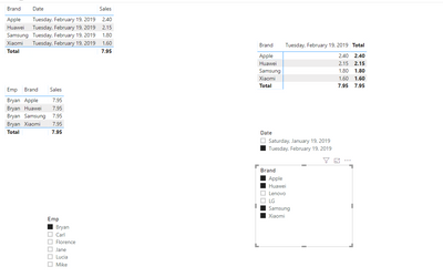
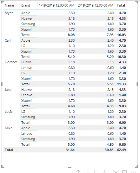
So we can get the results using filters. Just need some measures.

[smpa01]

@AshleyMartinez  my approach is following

A. Create a table as following called NewTbl

NewTbl = 
VAR _x = SELECTCOLUMNS (
    'Table 2',
    "Name", 'Table 2'[City Agent],
    "Brand", 'Table 2'[Brand]
)
VAR _y = SELECTCOLUMNS (
    'Table 2',
    "Name", 'Table 2'[Country Agent],
    "Brand", 'Table 2'[Brand]
)
VAR _z = SELECTCOLUMNS (
    'Table 2',
    "Name", 'Table 2'[Head of Account],
    "Brand", 'Table 2'[Brand]
)
VAR _a= SELECTCOLUMNS (
    'Table 2',
    "Name", 'Table 2'[Region Agent],
    "Brand", 'Table 2'[Brand]
)
 VAR _t= DISTINCT
                 (
                   UNION(_x,_y,_z,_a)
                 )
          
VAR _d= DISTINCT('Table 1'[Date])
VAR _cross = CROSSJOIN(_t,_d)
RETURN _cross

B.  Create a calculated column as following

Sales = LOOKUPVALUE('Table 1'[Sales],'Table 1'[Brand],NewTbl[Brand],'Table 1'[Date],NewTbl[Date])

 which gives the following

I am very interested to see now to see if this can be solved by creating a measure though.

[Nathaniel_C]

Hi @AshleyMartinez ,

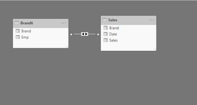
So, you say that you have created tables to link these two tables, but you are not successful.

How about Brand to Brand like this? 

Can you give us a picture of your model?

@Nathaniel_C 

[Nathaniel_C]

@AshleyMartinez ,

If you drop the new sales person column into the table such as "Mike" and filter out the blanks, and drop the "Mike" as a slicer you can then click on the company, and see "Mike" sales for the company.

Hope this helps your report,

If this solves your issues, please mark it as the solution, so that others can find it easily. Kudos are nice too.
Nathaniel

[Nathaniel_C]

@AshleyMartinez ,

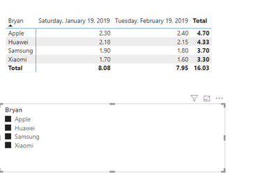
Created a column in PBI, although you would be better off in PQ, an If statement shown below. You still have some work to do,

Filter out the empty rows using the visual filter.

Let me know if you have any questions,

If this solves your issues, please mark it as the solution, so that others can find it easily. Kudos are nice too.
Nathaniel

Bryan = IF(Brand[City Agent] = "Bryan" || Brand[Country Agent] ="Bryan" || Brand[Head of Account] = "Bryan" || Brand[Region Agent] = "Bryan",Brand[Brand])

f

[AshleyMartinez]

Hi @Nathaniel_C , thanks for the early reply!

The thing is that my actual data base is very large, I have more than 70 sales persons and I'd like to automate the query. The problem with hardcode like typing "Bryan" in the DAX formula is that i'll have to create it 70 times for each worker.