Get Fabric certified for FREE!
Don't miss your chance to take the Fabric Data Engineer (DP-600) exam for FREE! Find out how by attending the DP-600 session on April 23rd (pacific time), live or on-demand.
Learn more- Power BI forums
- Get Help with Power BI
- Desktop
- Service
- Report Server
- Power Query
- Mobile Apps
- Developer
- DAX Commands and Tips
- Custom Visuals Development Discussion
- Health and Life Sciences
- Power BI Spanish forums
- Translated Spanish Desktop
- Training and Consulting
- Instructor Led Training
- Dashboard in a Day for Women, by Women
- Galleries
- Data Stories Gallery
- Themes Gallery
- Contests Gallery
- QuickViz Gallery
- Quick Measures Gallery
- Visual Calculations Gallery
- Notebook Gallery
- Translytical Task Flow Gallery
- TMDL Gallery
- R Script Showcase
- Webinars and Video Gallery
- Ideas
- Custom Visuals Ideas (read-only)
- Issues
- Issues
- Events
- Upcoming Events
Next up in the FabCon + SQLCon recap series: The roadmap for Microsoft SQL and Maximizing Developer experiences in Fabric. All sessions are available on-demand after the live show. Register now
- Power BI forums
- Forums
- Get Help with Power BI
- Desktop
- Re: Conditional Formatting Slicer
- Subscribe to RSS Feed
- Mark Topic as New
- Mark Topic as Read
- Float this Topic for Current User
- Bookmark
- Subscribe
- Printer Friendly Page
- Mark as New
- Bookmark
- Subscribe
- Mute
- Subscribe to RSS Feed
- Permalink
- Report Inappropriate Content
Conditional Formatting Slicer
Hi All,
It may be confusing the way i'm explaining, but the requirement is like below..
I have source in excel which has data in region wise Actual and Target for the whole year of 2017.. we have separate column for each month. (Below snip for reference)
I have unpivot the whole months column and showing the values in Matrix visual.
Here scenario is like, If ACT is below TGT then the value should show Red and if the ACT is >= then its Green for certain KPI for ex, consider AAA and BBB. For CCC and DDD if the ACT is <= TGT then it should be Green and if ACT > TGT then it should be Red..
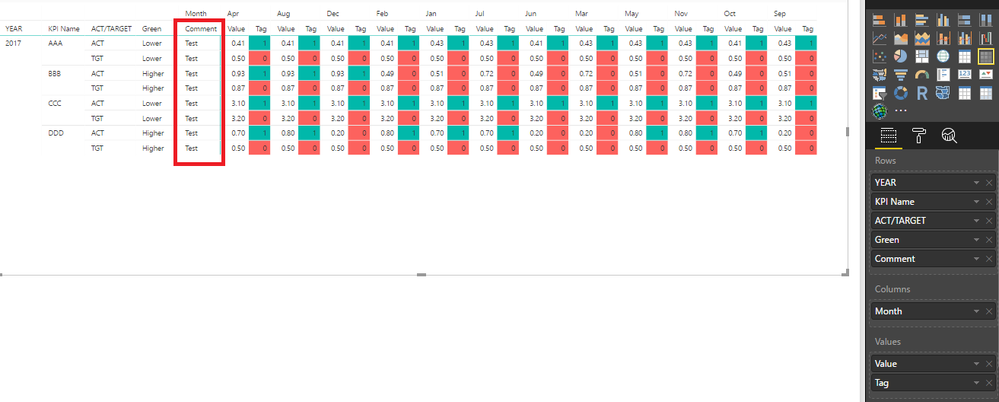
Somehow we have created the measure and put next to the value (Combined Months) column. (Below snip for reference)
Column green is based on KPI table, which has columns like KPI_ID, KPI_Desc, Green (Higher/Lower).. Higher means Act above the TGT, Lower means Act below the TGT (like i explained the Green and Red appearance scenario above).
Now where i'm struck is, we need a slicer to choose only Red KPI's i.e., wherever the Red color appear in that above image only visible rest should be blank or hide.
Many Thanks in Advance..
Hope you all understand my requirement.
@MattAllington @Baskar @Sean @Anonymous
Solved! Go to Solution.
- Mark as New
- Bookmark
- Subscribe
- Mute
- Subscribe to RSS Feed
- Permalink
- Report Inappropriate Content
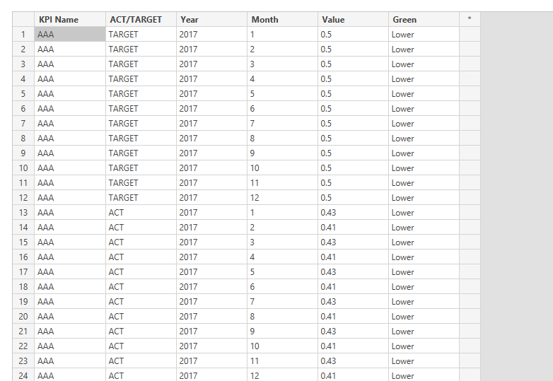
Firstly, you should pivot your months into one column:
Then create a calculated column to assign value (1 or 0) when achieving target or not.
Tag =
var CurrentTarget = LOOKUPVALUE('KPI'[Value],'KPI'[KPI Name],'KPI'[KPI Name],'KPI'[Year],'KPI'[Year],'KPI'[Month],'KPI'[Month],'KPI'[ACT/TARGET],"TARGET")
return
SWITCH('KPI'[Green],"Lower",IF('KPI'[Value]<CurrentTarget,1,0),"Higher",IF('KPI'[Value]>CurrentTarget,1,0))
Now you can create a matrix and apply conditional formatting on Tag column.
You can apply a slicer on Tag column to filter Red or Green.
Regards,
- Mark as New
- Bookmark
- Subscribe
- Mute
- Subscribe to RSS Feed
- Permalink
- Report Inappropriate Content
Hi All,
I want to do something the same as the problem discussed here but my scenario is a bit different. I am having three different columns as shown in the image and the condition has been applied to all three. Now I want to have a button or slicer which I click that should only show the red color only.
Thanks in advance.
- Mark as New
- Bookmark
- Subscribe
- Mute
- Subscribe to RSS Feed
- Permalink
- Report Inappropriate Content
Firstly, you should pivot your months into one column:
Then create a calculated column to assign value (1 or 0) when achieving target or not.
Tag =
var CurrentTarget = LOOKUPVALUE('KPI'[Value],'KPI'[KPI Name],'KPI'[KPI Name],'KPI'[Year],'KPI'[Year],'KPI'[Month],'KPI'[Month],'KPI'[ACT/TARGET],"TARGET")
return
SWITCH('KPI'[Green],"Lower",IF('KPI'[Value]<CurrentTarget,1,0),"Higher",IF('KPI'[Value]>CurrentTarget,1,0))
Now you can create a matrix and apply conditional formatting on Tag column.
You can apply a slicer on Tag column to filter Red or Green.
Regards,
- Mark as New
- Bookmark
- Subscribe
- Mute
- Subscribe to RSS Feed
- Permalink
- Report Inappropriate Content
Hi @v-sihou-msft,
Could you also help me on the below issue i have faced, actually i have 13 columns (12months and 1 comment).
So when i unpivot all columns (13) it was done because i dont have any values in comment column (Only Null). Now when i try to include some text and try the same, it pops the below error
Final stage i'm struck.
Many Thanks
- Mark as New
- Bookmark
- Subscribe
- Mute
- Subscribe to RSS Feed
- Permalink
- Report Inappropriate Content
I haven't gone through the entire thread, but...do you need to unpivot the Comment column? Could you just unpivot the months only?
- Mark as New
- Bookmark
- Subscribe
- Mute
- Subscribe to RSS Feed
- Permalink
- Report Inappropriate Content
Hi @MalS,
Actually i want to show the data in matrix visual, please check the above images. I did unpivot all months with comment column as well and it works because that time comment column had null values. after i put some testing data and refresh it i faced the datatype conversion error.. So i need to show the comment part after all months like below.
Jan Feb Mar.... Dec.. Comments
Hope you understand my requirement. if you want i ll give further explanation.
Thanks,
THiyaga
- Mark as New
- Bookmark
- Subscribe
- Mute
- Subscribe to RSS Feed
- Permalink
- Report Inappropriate Content
Yes, but you could just unpivot the months (not the Comment column).
Then when you create the matrix, you can add the Comment field to the rows section of the matrix.
- Mark as New
- Bookmark
- Subscribe
- Mute
- Subscribe to RSS Feed
- Permalink
- Report Inappropriate Content
No @MalS,
User requirement is to see last... Actually i did Mals but not in proper way..
Unpivot all months and create a calculated column to show only comments if the month is Dec else blank(). So the comment will appear only after dec. then i resize all the columns except Dec comment section and rename it.
Many Thanks for your efforts and work around Mals.
Thanks a lot.
- Mark as New
- Bookmark
- Subscribe
- Mute
- Subscribe to RSS Feed
- Permalink
- Report Inappropriate Content
Alternatively, you could unpivot the Comments column with the months, then make sure the resulting Values column had a data type of Text. Then, instead of summarizing the Value field using sum, min , max (or whatever you used originally), you should be able to summarize it using 'First' (which will work on a text field).
- Mark as New
- Bookmark
- Subscribe
- Mute
- Subscribe to RSS Feed
- Permalink
- Report Inappropriate Content
Hi @v-sihou-msft,
Thank you for timely help and it works what i expected... Really Great and Many thanks
- Mark as New
- Bookmark
- Subscribe
- Mute
- Subscribe to RSS Feed
- Permalink
- Report Inappropriate Content
Hi @v-sihou-msft,
Yeah i have found why the error appears, it retrieves lot of records with same names, so i have added other two columns in lookup now it works fine.
But i need to show the Target row as blank, so i have tried following measure, but it gives me an error, could you sort it out.
Many Thanks,
Cond_Form =
Var _Target = LOOKUPVALUE(Input[Value],Input[KPI],Input[KPI],Input[YEAR],Input[YEAR],Input[Months],Input[Months],Input[Category],Input[Category],Input[BG Name],Input[BG Name],Input[Site],Input[Site],Input[ACT/TARGET],"TGT")
Var _TGT = VALUES(Input[ACT/TARGET])
Return
	IF(_TGT = "TGT",BLANK(),
		SWITCH(Input[Green],"Lower",IF(Input[Value] <= _Target,1,0),"Higher",IF(Input[Value]>=_Target,1,0)))
- Mark as New
- Bookmark
- Subscribe
- Mute
- Subscribe to RSS Feed
- Permalink
- Report Inappropriate Content
Hi @v-sihou-msft,
Really very happy to see the response for this query,
I have did all the steps you have mentioned, but i get the below error while creating calc column
"A table of multiple values was supplied where a single value was expected."
Am i did anything wrong here?
- Mark as New
- Bookmark
- Subscribe
- Mute
- Subscribe to RSS Feed
- Permalink
- Report Inappropriate Content
Helpful resources

New to Fabric Survey
If you have recently started exploring Fabric, we'd love to hear how it's going. Your feedback can help with product improvements.

Power BI DataViz World Championships - June 2026
A new Power BI DataViz World Championship is coming this June! Don't miss out on submitting your entry.

Join our Fabric User Panel
Share feedback directly with Fabric product managers, participate in targeted research studies and influence the Fabric roadmap.

| User | Count |
|---|---|
| 48 | |
| 43 | |
| 39 | |
| 19 | |
| 17 |
| User | Count |
|---|---|
| 69 | |
| 63 | |
| 32 | |
| 30 | |
| 23 |


