Join us at FabCon Vienna from September 15-18, 2025
The ultimate Fabric, Power BI, SQL, and AI community-led learning event. Save €200 with code FABCOMM.
Get registeredEnhance your career with this limited time 50% discount on Fabric and Power BI exams. Ends August 31st. Request your voucher.
- Microsoft Fabric Community
- Fabric community blogs
- Power BI Community Blog
- Income Statement Analysis: Part 1 of 5
- Subscribe to RSS Feed
- Mark as New
- Mark as Read
- Bookmark
- Subscribe
- Printer Friendly Page
- Report Inappropriate Content
- Subscribe to RSS Feed
- Mark as New
- Mark as Read
- Bookmark
- Subscribe
- Printer Friendly Page
- Report Inappropriate Content
____________________
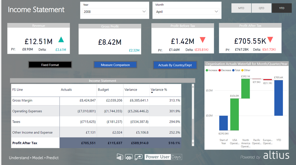
In this 5 part series, we walk through the steps required to build out the first page of the Income Statement Report here.
The topics covered in these walkthroughs include:
- Part 1: Connecting to Data (Folder Containing CSVs), Importing into Power BI
- Part 2: Creating the base measures and an Income Statement Matrix visual
______________
The scenario here is that we have monthly finance transactional data CSV files for each month from Jan 2007 to May 2008 (e.g. extracts from a ERP system) which we need to combine and analyze, bringing in the latest data on a monthly basis and showing MTD/QTD/YTD performance as well as a comparison to the prior year.
This is a common requirement in Finance and has typically been achieved with Excel using macros to combine files, lookup formulas to bring all the data into one wide table and external links to other files where historical data volumes are large and/or scattered across multiple files. Even with the use of macros, this process is typically still quite manual, time-consuming and error-prone. Individuals work on their own versions of spreadsheets which leads to a lack of governance/version control; the reporting is also typically quite static and difficult to draw real action-driven insights from.
In this series of blog posts, I will show run through building out an interactive Income Statement report in Power BI and the benefits of doing so, with step by step instructions for building out the report along with the rationale for each step.
1 Extract and review the Files
Extract the contents of the zip file attached in this blog post to a local folder on your machine. The source files in the Finance Data folder consist of the following:
- Monthly Results -> CSVs 35 monthly CSV files covering the period from July 2005 to May 2008. Each file contains transactions for the month with the following columns:
- DateKey: The first of the month in YYYYMMDD format (e.g. 20050701)
- MonthValue: The month in YYYYMM format (e.g. 200507)
- Organisation Key: The ID that relates to the Organisations sheet in the Reference data file (e.g. ID 8 relates to Organisation ‘Canadian Division’)
- Department Key: The ID that relates to the Departments sheet in the Reference data file (e.g. ID 6 relates to the department ‘Research and Development’)
- ScenarioKey: The ID that relates to the Scenarios sheet in the Reference data file (ID 1 relates to Actuals, 2 to Budget)
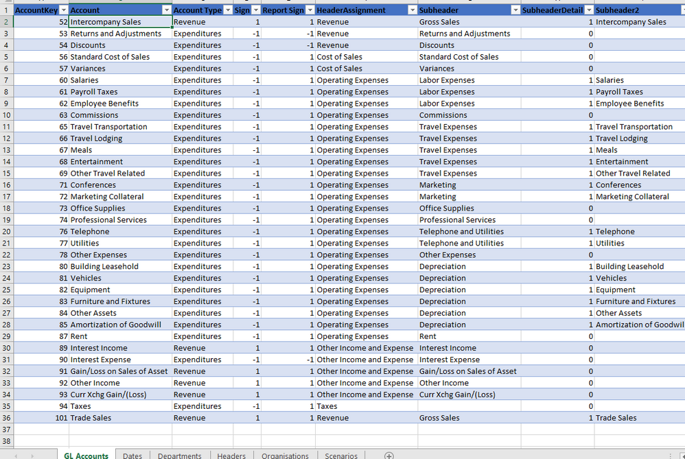
- Account Key: The GL Account ID that relates to the GL Accounts sheet in the Reference data file (e.g. GL Account 52 relates to Intercompany Sales; the GL Accounts sheet has details of each GL account e.g. the Account Type [Revenue/Expenditures], SubHeader, SubHeader2)
- Amount The amount of the transaction in local currency (The currency which relates to the department)
- Amount USD: The amount of the transaction in USD
- New Monthly File: A transaction file for June 2008, which we can copy into the Monthly Results folder and have it automatically picked up by Power BI
- Reference Data: An excel file with 6 worksheets, each for a different set of Reference data linked to in the transactional files.
If working with this data in Excel, we would have to combine all the monthly transaction data into a single file (if possible with the data volumes) in order to be able to analyze over time, and then use lookup formulas to bring in all the required reference data columns. We could then link this wide table into a fixed format Income statement report in Excel, and/or perform Pivot table analysis and graphs.
With Power BI, however, we can combine the transaction files automatically by connecting to the Monthly Results folder as our data source – each time the data is refreshed (up to 8 times per day with Power BI Pro) it will automatically pick up and combine all the files in that folder as well as apply any transformations required.
We can also keep the data tables (the transaction data and all the reference data) separate rather than having to combine them into one wide table. This is a more performant and efficient way of querying data and allows us to perform the type of analysis that we wouldn’t be able to if it were all in one table. (We will be organising our data tables in what is known as a star schema – see here for an article describing why it is required for more complex analysis).
2 Create a Parameter
Whilst we can just select the folder connector straight away from the data sources list and enter the folder path of the Monthly Results folder, we will instead first create a parameter with the folder path and use this in the connector instead.
Parameters in the Query editor (not to be confused with what-if parameters in the report view) are a way of storing values which are then referred to in one or more transformation steps. For example if this whole report was to be specific to only one particular region (though the data source contains data for all regions), you could store the required region value as a parameter and then refer to this when applying a filter on the data.
In this scenario, it is a good idea to store the folder path as a parameter because it refers to a path on your machine; if someone else opens the PBIX file on their machine instead, the folder path specified may not exist and they will need to update it to where those files are stored on their machine. Rather than updating the code in individual queries, they can just change the parameter value and any queries that refer to this folder path will then automatically reflect this updated value.
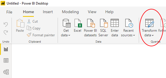
We start by creating a new report in Power BI Desktop and going to the query editor by clicking on ‘Transform Data’ under the Home Tab of the ribbon:
In Windows explorer, navigate to the folder where you saved the zip file contents in Step 1 above
From this folder navigate to the folder “\Finance Data\Monthly Results\CSVs” and copy the full folder path from the explorer bar
Back in the query editor in Power BI, click on Manage Parameters -> New Parameter
Give the parameter the name FolderPath, keep the type as Any and set the value to the folder you navigated to above and then press OK:
3 Connect to the Monthly Results Folder
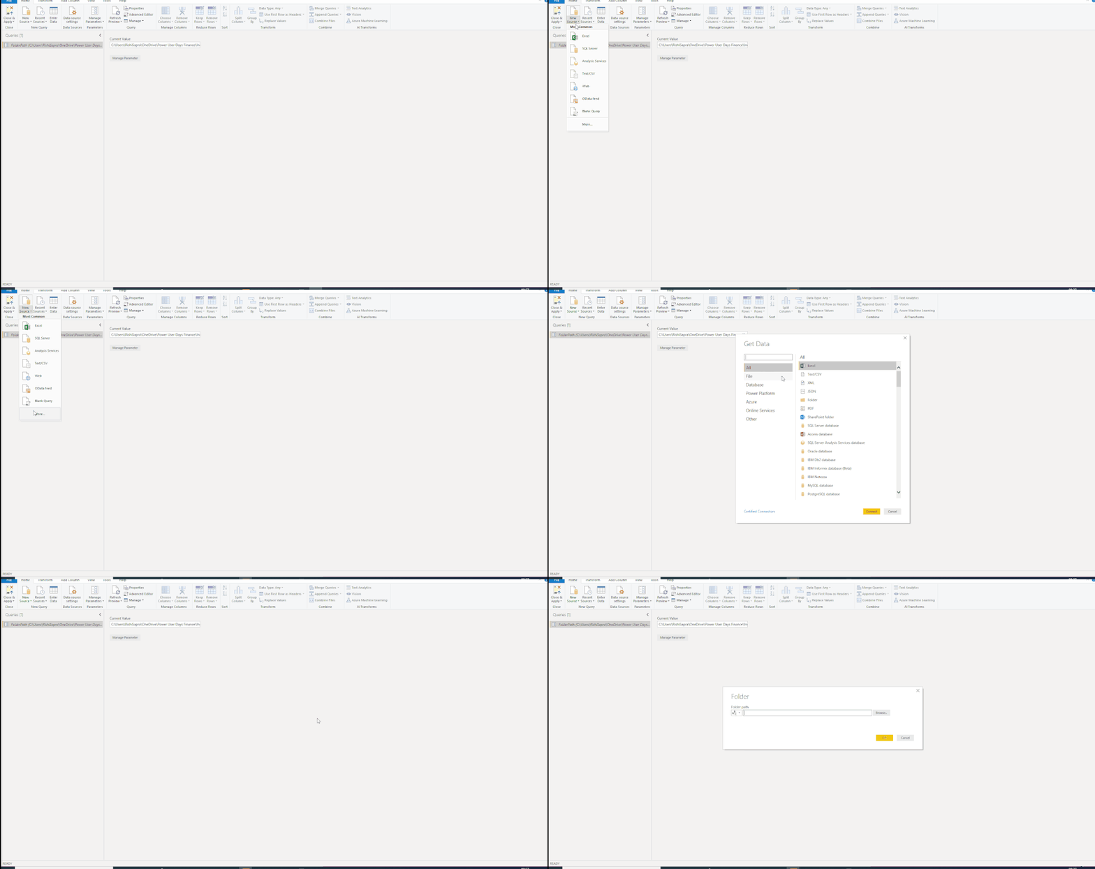
Click on ‘New Source’ in the Home tab of the query editor window and navigate to More... -> Folder (Under All) and then click connect:
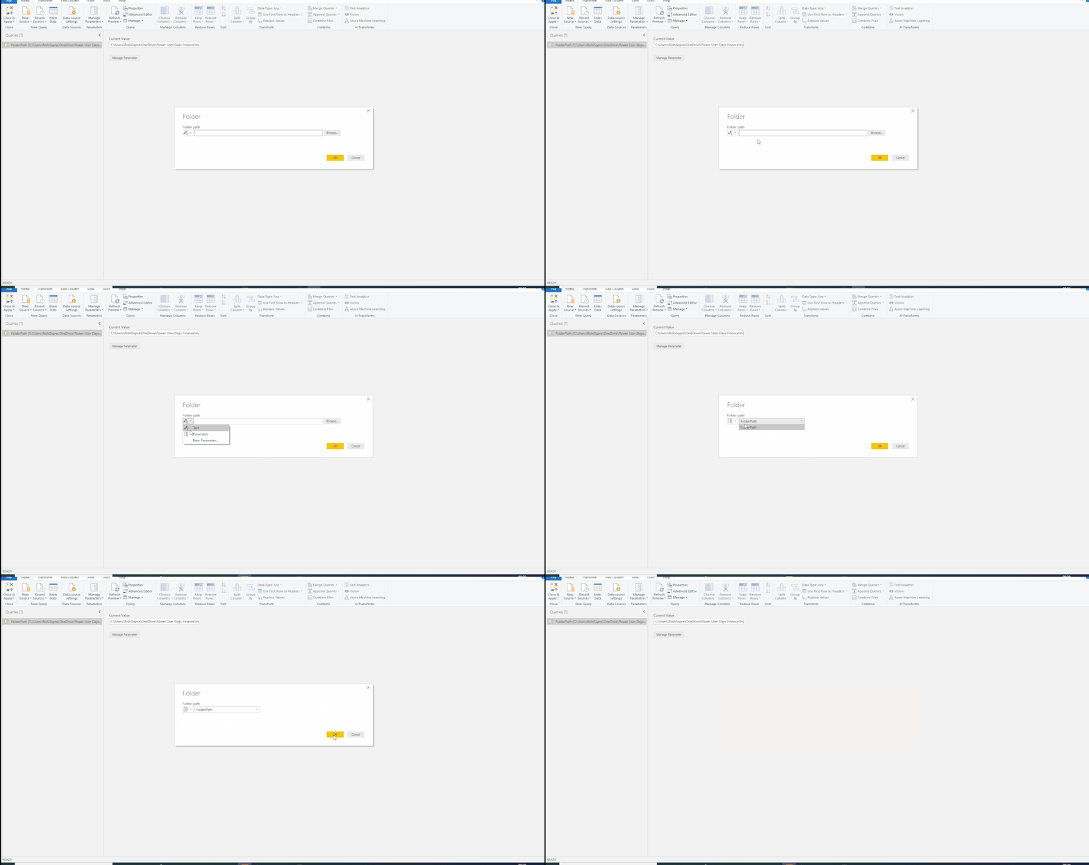
Click on the drop down next to the ABC box, select Parameter and ensure that the FolderPath parameter is selected then click ok:
Click on ‘Combine and Transform Data’ in the dialog box that shows up and accept the default options for combining:
By viewing the queries in the blade on the left-hand side of the screen, you will see that this step has generated a number of queries including a Sample File, a parameter linking to this Sample File and a Transform File function. The sample file is the first file in the folder (default option chosen above) which defines the format of all the files – each file in the folder will have to match the format (No of columns, data types) of this first file. The function is for any transformations that are required to be applied to each file before they are combined. By default, the only step in here is to promote headers (so that the header row isn’t repeated each time); if there are other transformations required you could modify this function or define your own.
4 Apply Transformations to the Combined Data
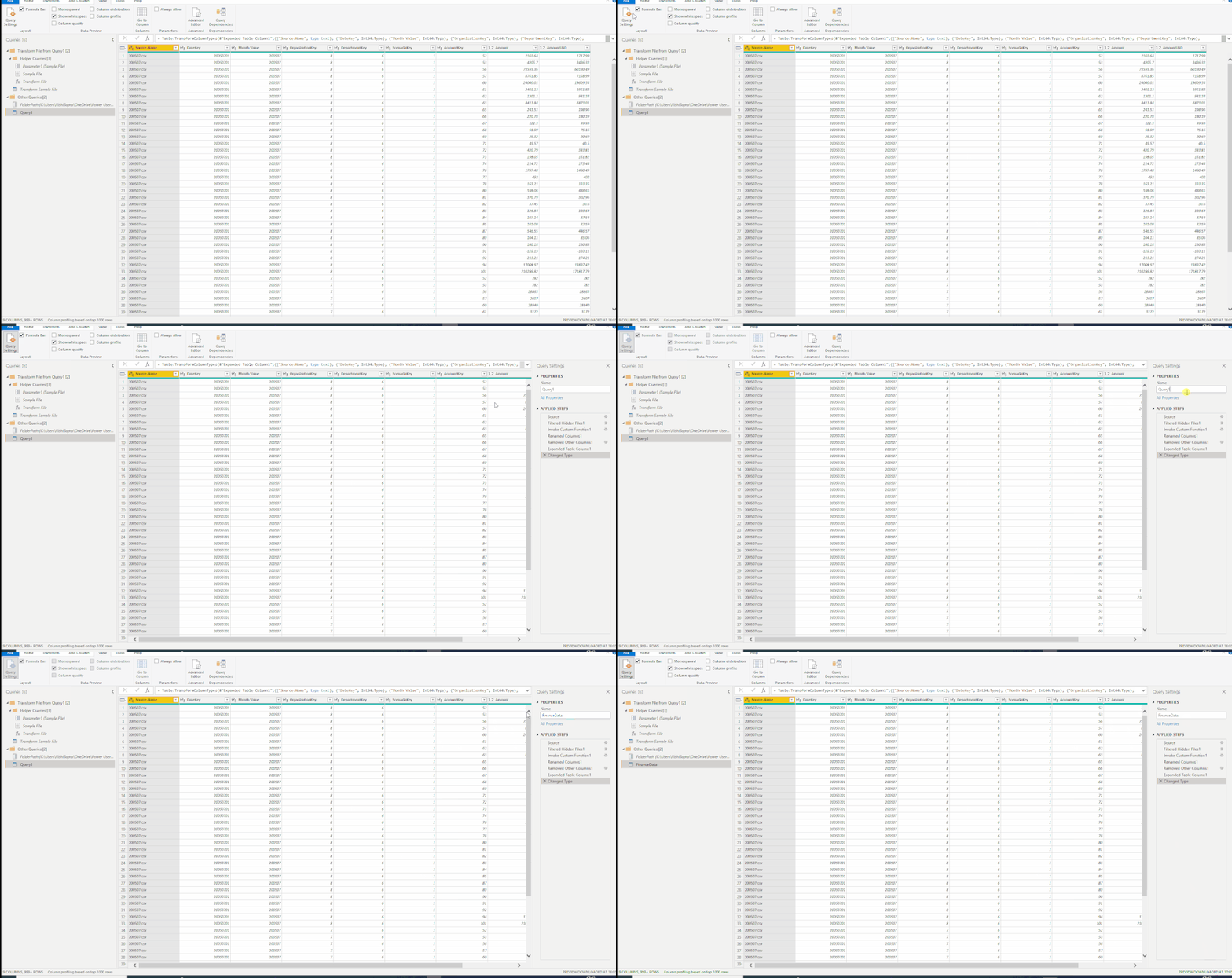
The Query with the combined data from all the CSV files is in a query called ‘Query1’. Rename this to something more sensible (e.g. FInanceData) by clicking on the Name under the Query settings and changing the value. Note that if this pane is not visible, it can be made so by selecting ‘Query settings’ from the view pane:
The query settings pane shows all the transformation steps applied. Clicking on a step will show the data with all steps up until that point applied; steps can be deleted or moved up/down, though be careful of doing this as certain steps might require prior steps to have taken place (e.g. the renaming of a new column can’t happen until that column is created!).
Combining the data above already created a number of steps automatically in Query1 – e.g. applying the transformation function to each file, using ‘Expand Contents’ to combine the data and changing the data types. It is often better to delete the automatic data type change step and set the data types yourself at the end as a last step before closing. However, in this case we aren’t really applying any further transformations and the data types have been applied correctly.
The only transformation step we can apply ourselves is to remove columns which are not needed – e.g. in this case we don’t need the first column ‘Source.Name’. With this column selected, right click on the column and select ‘Remove’.
5 Bring in the Reference Data
We now need to bring in the Reference data worksheets in the ‘Reference Data’ Excel file – e.g. the list of Accounts and the list of Organisations.
To do this, select ‘New Source’ in Home ribbon and Navigate to the Excel option.
Navigate to the Reference Data.xlsx file saved in the folder path Finance Data\Reference Tables
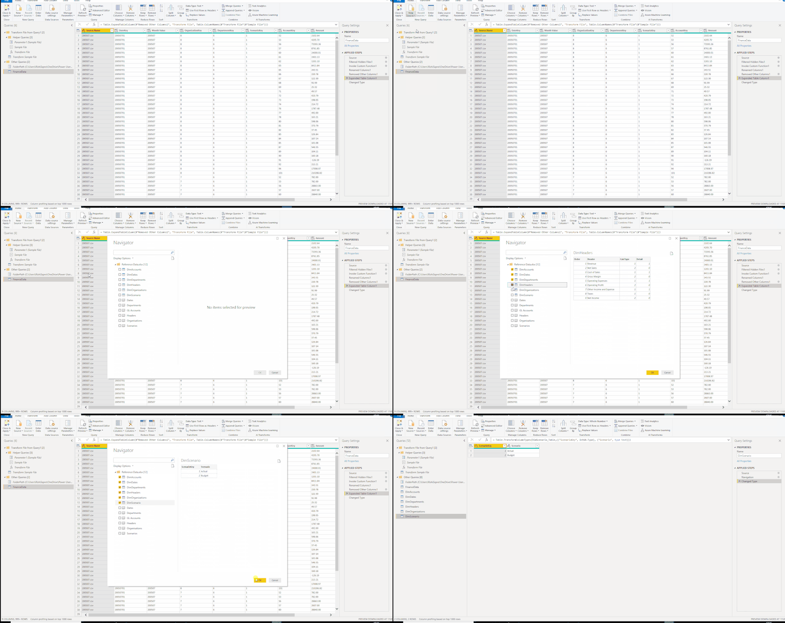
In the Navigator option that comes up , select all of the tables (denoted with a table icon, not also selecting those with the worksheet icon as this would double up the data) and then click OK:
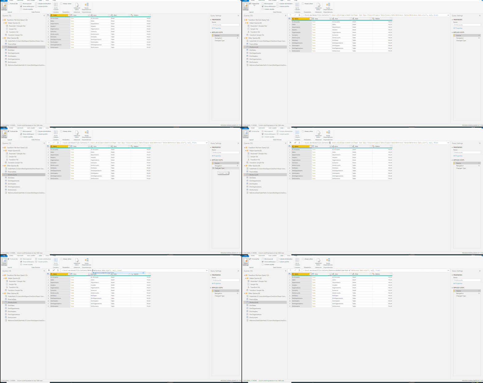
Note that the path of the Excel file has been hardcoded into the transformation steps which is something that we were trying to avoid with the Finance data. To remedy this, we can create another parameter e.g. called ReferenceDataFolderPath and then manually update the code generated by us brining in the Excel file to refer to the new parameter instead.
Note that you can edit/tweak the M code that is automatically generated by the Query Editor UI either in the formula bar (where this is not visible, select the checkbox from the ‘View’ tab of the ribbon) and/or from the Advanced Editor, accessible via the Home tab.
6 Organise Queries
It is good practice to organise your queries into folders called Query Groups.
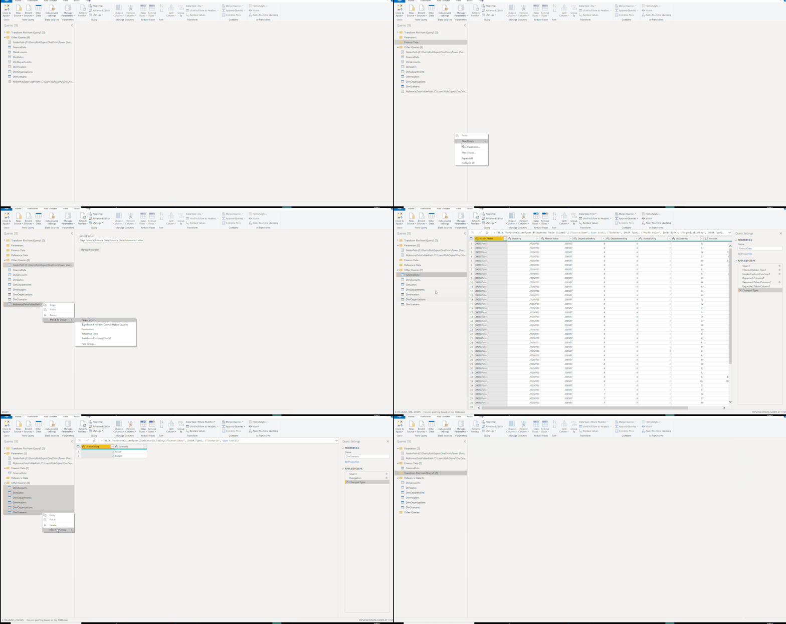
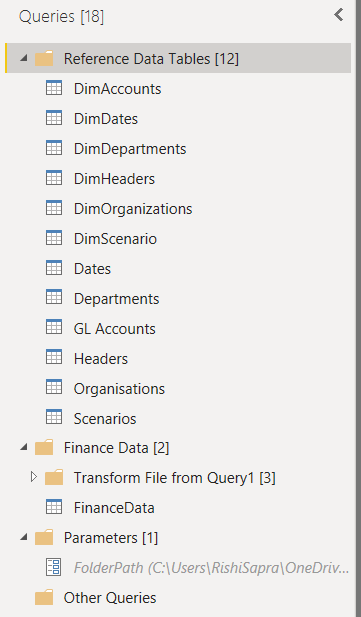
You can create the folders ‘Parameters’, ‘Finance Data’, ‘Reference Data’ by right clicking in the blank space under the list of queries and selecting ‘New Group’:
Then select the queries (for multiple queries holding shift and select), right click and select ‘Move to Group’ to move them into the correct folders:
7 Close
Click on ‘Close and Apply’ to bring all the data into Power BI:
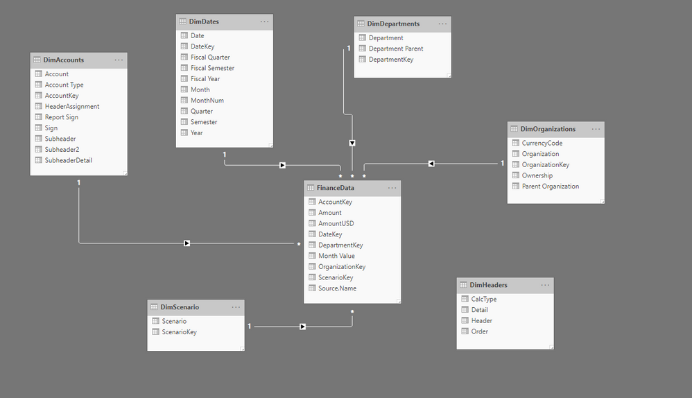
Navigate to the Model view in Power BI Desktop. Your data model view should now look something like this (with relationships autodetected):
You must be a registered user to add a comment. If you've already registered, sign in. Otherwise, register and sign in.
- 🏆 Power BI DataViz World Championships | EU Editi...
- How are Fabric Community Dataviz Contests Judged?
- Power BI Integration with Databricks
- 10 Power BI Tricks Every Analyst Should Know in 20...
- Document PBIP report using AI
- While Loop in M Language - In Short
- 🌟 Judges’ Favorites: Honoring More Standout Entri...
- 🎉 And the Winners Are… Celebrating the Best of th...
- 🎉Power BI Turns 10! Grab your digital swag!
- Level Up Your Reports: Mastering Power BI Performa...
-
Mayamiko
 on:
How are Fabric Community Dataviz Contests Judged?
- TharunChalla on: Power BI Integration with Databricks
-
wardy912
 on:
Document PBIP report using AI
-
Meng
 on:
🌟 Judges’ Favorites: Honoring More Standout Entri...
-
LucasKoch2900
 on:
🎉 And the Winners Are… Celebrating the Best of th...
-
Leanore
 on:
🎉Power BI Turns 10! Grab your digital swag!
- sgunasekhar1 on: Level Up Your Reports: Mastering Power BI Performa...
-
 bhanu_gautam
on:
ISINSCOPE vs HASONEVALUE in Power BI: The Real Dif...
-
 v-agajavelly
on:
Button Slicer / How to Make Images as Slicers in P...
- lokesh0909 on: Unlocking the Power of Calculation Group - Beyond ...
-
How to
673 -
Tips & Tricks
650 -
Events
148 -
Support insights
121 -
Opinion
82 -
DAX
66 -
Power BI
65 -
Power Query
62 -
Power BI Dev Camp
45 -
Power BI Desktop
40 -
Roundup
37 -
Dataflow
23 -
Featured User Group Leader
21 -
Power BI Embedded
20 -
Time Intelligence
19 -
Tips&Tricks
18 -
PowerBI REST API
12 -
Data Protection
11 -
Power BI Service
8 -
Power Query Tips & Tricks
8 -
finance
8 -
Direct Query
7 -
Data Visualization
6 -
Python
6 -
Power BI REST API
6 -
Auto ML
6 -
financial reporting
6 -
Data Analysis
6 -
Power Automate
6 -
Machine Learning
5 -
Income Statement
5 -
Dax studio
5 -
powerbi
5 -
service
5 -
Power BI PowerShell
5 -
Bookmarks
4 -
Line chart
4 -
Group By
4 -
community
4 -
RLS
4 -
M language
4 -
Paginated Reports
4 -
External tool
4 -
Power BI Goals
4 -
Desktop
4 -
PowerShell
4 -
PowerApps
3 -
Tips and Tricks
3 -
Data Science
3 -
Azure
3 -
Data model
3 -
Conditional Formatting
3 -
Visualisation
3 -
Life Sciences
3 -
Administration
3 -
M code
3 -
Visuals
3 -
SQL Server 2017 Express Edition
3 -
R script
3 -
Aggregation
3 -
Webinar
3 -
calendar
3 -
Gateways
3 -
R
3 -
M Query
3 -
CALCULATE
3 -
R visual
3 -
Reports
3 -
Visualization
2 -
Power BI Challenge
2 -
Query Parameter
2 -
SharePoint
2 -
Power BI Installation and Updates
2 -
How Things Work
2 -
Tabular Editor
2 -
rank
2 -
ladataweb
2 -
Troubleshooting
2 -
Date DIFF
2 -
Transform data
2 -
Healthcare
2 -
Incremental Refresh
2 -
Number Ranges
2 -
Query Plans
2 -
Power BI & Power Apps
2 -
Random numbers
2 -
Day of the Week
2 -
Custom Visual
2 -
VLOOKUP
2 -
pivot
2 -
calculated column
2 -
M
2 -
hierarchies
2 -
Power BI Anniversary
2 -
Language M
2 -
inexact
2 -
Date Comparison
2 -
Power BI Premium Per user
2 -
Forecasting
2 -
REST API
2 -
Editor
2 -
Split
2 -
measure
2 -
Microsoft-flow
2 -
Paginated Report Builder
2 -
Working with Non Standatd Periods
2 -
powerbi.tips
2 -
Custom function
2 -
Reverse
2 -
PUG
2 -
Custom Measures
2 -
Filtering
2 -
Row and column conversion
2 -
Python script
2 -
Nulls
2 -
DVW Analytics
2 -
parameter
2 -
Industrial App Store
2 -
Week
2 -
Date duration
2 -
Formatting
2 -
Weekday Calendar
2 -
Support insights.
2 -
construct list
2 -
slicers
2 -
SAP
2 -
Power Platform
2 -
Workday
2 -
external tools
2 -
index
2 -
RANKX
2 -
Date
2 -
PBI Desktop
2 -
Date Dimension
2 -
Integer
2 -
Excel
1 -
Showcase
1 -
custom connector
1 -
Waterfall Chart
1 -
Power BI On-Premise Data Gateway
1 -
patch
1 -
Top Category Color
1 -
A&E data
1 -
Previous Order
1 -
Substring
1 -
Wonderware
1 -
Power M
1 -
Format DAX
1 -
Custom functions
1 -
accumulative
1 -
DAX&Power Query
1 -
Premium Per User
1 -
GENERATESERIES
1 -
Report Server
1 -
Audit Logs
1 -
analytics pane
1 -
step by step
1 -
Top Brand Color on Map
1 -
Tutorial
1 -
Previous Date
1 -
XMLA End point
1 -
color reference
1 -
Date Time
1 -
Marker
1 -
Lineage
1 -
CSV file
1 -
conditional accumulative
1 -
Matrix Subtotal
1 -
Check
1 -
null value
1 -
Show and Tell
1 -
Cumulative Totals
1 -
Report Theme
1 -
Bookmarking
1 -
oracle
1 -
mahak
1 -
pandas
1 -
Networkdays
1 -
Button
1 -
Dataset list
1 -
Keyboard Shortcuts
1 -
Fill Function
1 -
LOOKUPVALUE()
1 -
Tips &Tricks
1 -
Plotly package
1 -
Sameperiodlastyear
1 -
Office Theme
1 -
matrix
1 -
bar chart
1 -
Measures
1 -
powerbi argentina
1 -
Canvas Apps
1 -
total
1 -
Filter context
1 -
Difference between two dates
1 -
get data
1 -
OSI
1 -
Query format convert
1 -
ETL
1 -
Json files
1 -
Merge Rows
1 -
CONCATENATEX()
1 -
take over Datasets;
1 -
Networkdays.Intl
1 -
refresh M language Python script Support Insights
1 -
Tutorial Requests
1 -
Governance
1 -
Fun
1 -
Power BI gateway
1 -
gateway
1 -
Elementary
1 -
Custom filters
1 -
Vertipaq Analyzer
1 -
powerbi cordoba
1 -
Model Driven Apps
1 -
REMOVEFILTERS
1 -
XMLA endpoint
1 -
translations
1 -
OSI pi
1 -
Parquet
1 -
Change rows to columns
1 -
remove spaces
1 -
Get row and column totals
1 -
Retail
1 -
Power BI Report Server
1 -
School
1 -
Cost-Benefit Analysis
1 -
DIisconnected Tables
1 -
Sandbox
1 -
Honeywell
1 -
Combine queries
1 -
X axis at different granularity
1 -
ADLS
1 -
Primary Key
1 -
Microsoft 365 usage analytics data
1 -
Randomly filter
1 -
Week of the Day
1 -
Azure AAD
1 -
query
1 -
Dynamic Visuals
1 -
KPI
1 -
Intro
1 -
Icons
1 -
ISV
1 -
Ties
1 -
unpivot
1 -
Practice Model
1 -
Continuous streak
1 -
ProcessVue
1 -
Create function
1 -
Table.Schema
1 -
Acknowledging
1 -
Postman
1 -
Text.ContainsAny
1 -
Power BI Show
1 -
Get latest sign-in data for each user
1 -
Power Pivot
1 -
API
1 -
Kingsley
1 -
Merge
1 -
variable
1 -
Issues
1 -
function
1 -
stacked column chart
1 -
ho
1 -
ABB
1 -
KNN algorithm
1 -
List.Zip
1 -
optimization
1 -
Artificial Intelligence
1 -
Map Visual
1 -
Text.ContainsAll
1 -
Tuesday
1 -
help
1 -
group
1 -
Scorecard
1 -
Json
1 -
Tops
1 -
financial reporting hierarchies RLS
1 -
Featured Data Stories
1 -
MQTT
1 -
Custom Periods
1 -
Partial group
1 -
Reduce Size
1 -
FBL3N
1 -
Wednesday
1 -
Q&A
1 -
Quick Tips
1 -
data
1 -
PBIRS
1 -
Usage Metrics in Power BI
1 -
Multivalued column
1 -
Pipeline
1 -
Path
1 -
Yokogawa
1 -
Dynamic calculation
1 -
Data Wrangling
1 -
native folded query
1 -
transform table
1 -
UX
1 -
Cell content
1 -
General Ledger
1 -
Thursday
1 -
update
1 -
Table
1 -
Natural Query Language
1 -
Infographic
1 -
automation
1 -
Prediction
1 -
newworkspacepowerbi
1 -
Performance KPIs
1 -
HR Analytics
1 -
keepfilters
1 -
Connect Data
1 -
Financial Year
1 -
Schneider
1 -
dynamically delete records
1 -
Copy Measures
1 -
Friday
1 -
Training
1 -
Event
1 -
Custom Visuals
1 -
Free vs Pro
1 -
Format
1 -
Active Employee
1 -
Custom Date Range on Date Slicer
1 -
refresh error
1 -
PAS
1 -
certain duration
1 -
DA-100
1 -
bulk renaming of columns
1 -
Single Date Picker
1 -
Monday
1 -
PCS
1 -
Saturday
1 -
Slicer
1 -
Visual
1 -
forecast
1 -
Regression
1 -
CICD
1 -
Current Employees
1 -
date hierarchy
1 -
relationship
1 -
SIEMENS
1 -
Multiple Currency
1 -
Power BI Premium
1 -
On-premises data gateway
1 -
Binary
1 -
Power BI Connector for SAP
1 -
Sunday
1 -
Workspace
1 -
Announcement
1 -
Features
1 -
domain
1 -
pbiviz
1 -
sport statistics
1 -
Intelligent Plant
1 -
Circular dependency
1 -
GE
1 -
Exchange rate
1 -
Dendrogram
1 -
range of values
1 -
activity log
1 -
Decimal
1 -
Charticulator Challenge
1 -
Field parameters
1 -
deployment
1 -
ssrs traffic light indicators
1 -
SQL
1 -
trick
1 -
Scripts
1 -
Color Map
1 -
Industrial
1 -
Weekday
1 -
Working Date
1 -
Space Issue
1 -
Emerson
1 -
Date Table
1 -
Cluster Analysis
1 -
Stacked Area Chart
1 -
union tables
1 -
Number
1 -
Start of Week
1 -
Tips& Tricks
1 -
Theme Colours
1 -
Text
1 -
Flow
1 -
Publish to Web
1 -
Extract
1 -
Topper Color On Map
1 -
Historians
1 -
context transition
1 -
Custom textbox
1 -
OPC
1 -
Zabbix
1 -
Label: DAX
1 -
Business Analysis
1 -
Supporting Insight
1 -
rank value
1 -
Synapse
1 -
End of Week
1 -
Tips&Trick
1
- 07-27-2025 - 08-01-2025
- 07-20-2025 - 07-26-2025
- 07-13-2025 - 07-19-2025
- 07-06-2025 - 07-12-2025
- 06-29-2025 - 07-05-2025
- 06-22-2025 - 06-28-2025
- 06-15-2025 - 06-21-2025
- 06-08-2025 - 06-14-2025
- 06-01-2025 - 06-07-2025
- 05-25-2025 - 05-31-2025
- 05-18-2025 - 05-24-2025
- 05-11-2025 - 05-17-2025
- 05-04-2025 - 05-10-2025
- 04-27-2025 - 05-03-2025
- View Complete Archives
