FabCon is coming to Atlanta
Join us at FabCon Atlanta from March 16 - 20, 2026, for the ultimate Fabric, Power BI, AI and SQL community-led event. Save $200 with code FABCOMM.
Register now!- Power BI forums
- Get Help with Power BI
- Desktop
- Service
- Report Server
- Power Query
- Mobile Apps
- Developer
- DAX Commands and Tips
- Custom Visuals Development Discussion
- Health and Life Sciences
- Power BI Spanish forums
- Translated Spanish Desktop
- Training and Consulting
- Instructor Led Training
- Dashboard in a Day for Women, by Women
- Galleries
- Data Stories Gallery
- Themes Gallery
- Contests Gallery
- QuickViz Gallery
- Quick Measures Gallery
- Visual Calculations Gallery
- Notebook Gallery
- Translytical Task Flow Gallery
- TMDL Gallery
- R Script Showcase
- Webinars and Video Gallery
- Ideas
- Custom Visuals Ideas (read-only)
- Issues
- Issues
- Events
- Upcoming Events
The Power BI Data Visualization World Championships is back! Get ahead of the game and start preparing now! Learn more
- Power BI forums
- Forums
- Get Help with Power BI
- Desktop
- Conditional formatting based on bechmarks that dif...
- Subscribe to RSS Feed
- Mark Topic as New
- Mark Topic as Read
- Float this Topic for Current User
- Bookmark
- Subscribe
- Printer Friendly Page
- Mark as New
- Bookmark
- Subscribe
- Mute
- Subscribe to RSS Feed
- Permalink
- Report Inappropriate Content
Conditional formatting based on bechmarks that differ by columns
Hello,
I have a matrix with facilities listed in the rows and tests listed in the columns. The values in the middle of the table are a measure calculated as the number of times a facility exceeds the test divided by the total number of facilities taking the test.
Test A, B, C
Facility 1 - 33%, 0%, 77.27%
Facility 2 - 66.67%, 77.78%, 100%
Facility 3 - 56.67%, 0%, 33.33%
Test A has a benchmark of 50%, Test B has a benchmark of 70%, Test C has a benchmark of 30%.
I would like to apply conditional formatting to the cell values based on the bench of each column. I believe this can be achieved by adding conditional formatting by field value the formatting doesn't seem to apply in all situations.
Color = SWITCH(TRUE(),'APP'[Test]=A&&[AnswerStatus%]>.5, "#008000",
'APP'[Test]=B&&[AnswerStatus%]>.70, "#008000", 'APP'[Test]=C&&[AnswerStatus%]>.30, "#008000")
My ideal soltuion is:
Test A, B, C
Facility 1 - 33%, 0%, 77.27%
Facility 2 - 66.67%, 77.78%, 100%
Facility 3 - 56.67%, 0%, 33.33%
A bonus would be to even add an additional column that would be a count of the number of greens in a row.
Test A, B, C, COUNT_GREEN
Facility 1 - 33%, 0%, 77.27%, 1
Facility 2 - 66.67%, 77.78%, 100%, 3
Facility 3 - 56.67%, 0%, 33.33%, 2
Thanks so much in advance for the DAX genius 🙂
Ashley
Solved! Go to Solution.
- Mark as New
- Bookmark
- Subscribe
- Mute
- Subscribe to RSS Feed
- Permalink
- Report Inappropriate Content
Hi @Anonymous
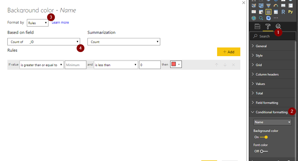
You need to go to FORMAT section (1).
There choose CONDITIONAL FORMATING (2).
Choose the field to format. Another window will pop up.
Choose RULES (3), and BASED ON FIELD - Will be the new calculated field (4).
In the example, I format NAME according to COUNT of IDs.
- Mark as New
- Bookmark
- Subscribe
- Mute
- Subscribe to RSS Feed
- Permalink
- Report Inappropriate Content
Hi @Anonymous
Are you missing a 'else' condition?
i.e.
Color = SWITCH(TRUE(),'APP'[Test]=A&&[AnswerStatus%]>.5, "#008000",
'APP'[Test]=B&&[AnswerStatus%]>.70, "#008000", 'APP'[Test]=C&&[AnswerStatus%]>.30, "#008000", "#ff0000")
Another way is, to create 3 calculated columns for each test result.
i.e.
Column_A_Result = IF(AnswerStatus>0.5,1,2)
Then format the column according to this number/column (1=green,2-red). And you can sum up the 1s (column_sum = SUM(Column_A_Result,Column_B_Result ,Column_C_Result ))
Good luck!
A
- Mark as New
- Bookmark
- Subscribe
- Mute
- Subscribe to RSS Feed
- Permalink
- Report Inappropriate Content
Thanks so much for the assist @Anonymous!
The else statement isn't needed with the switch. Instead, I added a >= and a < clause - but no dice.
Exploring the column_result option. If I want to format the column according to this number/column (1=green,2-red), where in PowerBI can I apply the format to each column individually?
- Mark as New
- Bookmark
- Subscribe
- Mute
- Subscribe to RSS Feed
- Permalink
- Report Inappropriate Content
Hi @Anonymous
You need to go to FORMAT section (1).
There choose CONDITIONAL FORMATING (2).
Choose the field to format. Another window will pop up.
Choose RULES (3), and BASED ON FIELD - Will be the new calculated field (4).
In the example, I format NAME according to COUNT of IDs.
Helpful resources

Power BI Dataviz World Championships
The Power BI Data Visualization World Championships is back! Get ahead of the game and start preparing now!

| User | Count |
|---|---|
| 40 | |
| 35 | |
| 34 | |
| 31 | |
| 28 |
| User | Count |
|---|---|
| 136 | |
| 102 | |
| 68 | |
| 66 | |
| 58 |


