Join us at the 2025 Microsoft Fabric Community Conference
March 31 - April 2, 2025, in Las Vegas, Nevada. Use code MSCUST for a $150 discount! Early bird discount ends December 31.
Register Now- Power BI forums
- Get Help with Power BI
- Desktop
- Service
- Report Server
- Power Query
- Mobile Apps
- Developer
- DAX Commands and Tips
- Custom Visuals Development Discussion
- Health and Life Sciences
- Power BI Spanish forums
- Translated Spanish Desktop
- Training and Consulting
- Instructor Led Training
- Dashboard in a Day for Women, by Women
- Galleries
- Community Connections & How-To Videos
- COVID-19 Data Stories Gallery
- Themes Gallery
- Data Stories Gallery
- R Script Showcase
- Webinars and Video Gallery
- Quick Measures Gallery
- 2021 MSBizAppsSummit Gallery
- 2020 MSBizAppsSummit Gallery
- 2019 MSBizAppsSummit Gallery
- Events
- Ideas
- Custom Visuals Ideas
- Issues
- Issues
- Events
- Upcoming Events
Be one of the first to start using Fabric Databases. View on-demand sessions with database experts and the Microsoft product team to learn just how easy it is to get started. Watch now
- Power BI forums
- Forums
- Get Help with Power BI
- DAX Commands and Tips
- Re: Is there sth wrong with summarize function?
- Subscribe to RSS Feed
- Mark Topic as New
- Mark Topic as Read
- Float this Topic for Current User
- Bookmark
- Subscribe
- Printer Friendly Page
- Mark as New
- Bookmark
- Subscribe
- Mute
- Subscribe to RSS Feed
- Permalink
- Report Inappropriate Content
Is there sth wrong with summarize function?
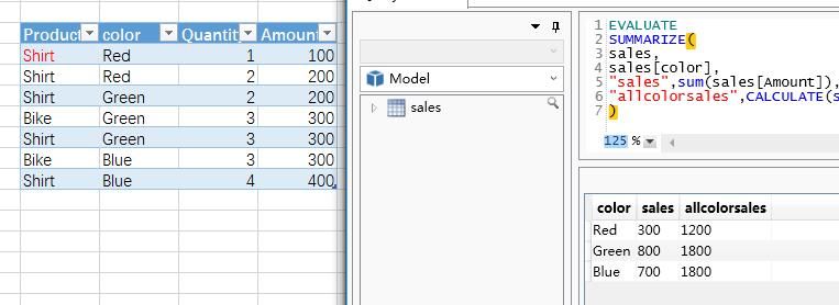
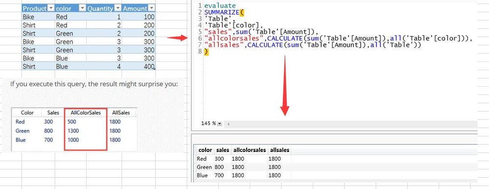
I Reproduce the scenario in http://www.sqlbi.com/articles/all-the-secrets-of-summarize/, but the answer is different.
anyone can explain it?
change the first product from bike to shirt, the answer is different:

Solved! Go to Solution.
- Mark as New
- Bookmark
- Subscribe
- Mute
- Subscribe to RSS Feed
- Permalink
- Report Inappropriate Content
Well, the Power Pivot engine in Excel 2016 is not the same as the one used by Excel 2013 (when Marco Russo wrote his article).
I have made a few tests, and here are my conclusions: this is a bug.
The long version is the behaviour no longer works as Marco Russo explained in his article. There is still an implicit filter but only on the first column in the table (at the time of creation).
If you create a new table with columns listed in this order: Quantity, Product, Color, Amount, like this:
| Quantity | Product | Color | Amount |
| 1 | Shirt | Red | 100 |
| 2 | Shirt | Red | 200 |
| 2 | Shirt | Green | 200 |
| 3 | Bike | Green | 300 |
| 3 | Shirt | Green | 300 |
| 3 | Bike | Blue | 300 |
| 4 | Shirt | Blue | 400 |
Your query should now return the following:
Color allcolorsales
Red 500
Green 1300
Blue 1300
Note that, according to my observations, what is relevant is the columns order when the table was created. Re-ordering the columns afterwards does not seem to change the results of the query. This is, in my opinion, a bug.
- Mark as New
- Bookmark
- Subscribe
- Mute
- Subscribe to RSS Feed
- Permalink
- Report Inappropriate Content
When Marco Russo wrote his article, the value returned (500) was:
Total of Amount for all rows with
Product = "Bike" and Quantity = 1 and Amount = 100
or
Product = "Shirt" and Quantity = 2 and Amount = 200
1200 is the total of Amount rows for all rows where Product = "Shirt".
The implicit filter seems to ignore the columns Quantity and Price.
Do you use Excel 2016?
- Mark as New
- Bookmark
- Subscribe
- Mute
- Subscribe to RSS Feed
- Permalink
- Report Inappropriate Content
yes,Laurent, I did it in excel2016 and also Power BI, the answer is equal.
Does different version of the tool make different answer?
- Mark as New
- Bookmark
- Subscribe
- Mute
- Subscribe to RSS Feed
- Permalink
- Report Inappropriate Content
Well, the Power Pivot engine in Excel 2016 is not the same as the one used by Excel 2013 (when Marco Russo wrote his article).
I have made a few tests, and here are my conclusions: this is a bug.
The long version is the behaviour no longer works as Marco Russo explained in his article. There is still an implicit filter but only on the first column in the table (at the time of creation).
If you create a new table with columns listed in this order: Quantity, Product, Color, Amount, like this:
| Quantity | Product | Color | Amount |
| 1 | Shirt | Red | 100 |
| 2 | Shirt | Red | 200 |
| 2 | Shirt | Green | 200 |
| 3 | Bike | Green | 300 |
| 3 | Shirt | Green | 300 |
| 3 | Bike | Blue | 300 |
| 4 | Shirt | Blue | 400 |
Your query should now return the following:
Color allcolorsales
Red 500
Green 1300
Blue 1300
Note that, according to my observations, what is relevant is the columns order when the table was created. Re-ordering the columns afterwards does not seem to change the results of the query. This is, in my opinion, a bug.
- Mark as New
- Bookmark
- Subscribe
- Mute
- Subscribe to RSS Feed
- Permalink
- Report Inappropriate Content
Hi Laurent,
I wish it was a bug, unfortunately it is only extremely hard to understand, starting by myself! It took me a while to find the correct answer 🙂
The behavior is indeed different in the 2016 version but, since I wrote that article, I learned a bit more about DAX, and we've been able to understand the topic of arbitrarily shaped sets. This lead me to define the problem in an easier way.
In reality, the problem of SUMMARIZE is nothing but the creation of arbitrarily shaped sets that are destroyed as a consequence of context transition. In fact, it is worth remembering that SUMMARIZE is the only function, AFAIK, that generates both a row context and a filter context. The row context is seldom used, still it is there. Thus, as soon as you call CALCULATE, you force context transition, and this is the source of the error (or... let us call it a "feature").
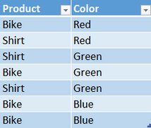
Why is this relevant? You can see the effect with a simpler table. The following one is a variation of the one used in the post. Please note that I removed the numeric columns and - in the last line - I put a Bike instead of a Shirt (this is VERY important, otherwise the problem does not show up; the previous dataset was too simple). Please note that there is NO Blue Shirt.
On this simpler model, you can run a variation of the original query:
EVALUATE
SUMMARIZE (
    Sales,
    Sales[Color],
    "Sales", COUNTROWS ( Sales ),
    "AllColorSales",
    CALCULATE (
        COUNTROWS ( Sales ),
        ALL ( Sales[Color] )
     ),
    "AllSales",
    CALCULATE (
        COUNTROWS ( Sales ),
        ALL ( Sales )
    )
)
I replaced SUM with COUNTROWS, because now I have a simpler model. The result, as you might guess, is wrong:
The last line, showing 4, is wrong. Why that? Because when you are on the BLUE row the filter context contains ( BLUE, BIKE ) and it is transformed into (BIKE), which contains 4 rows. When you are on Green, on the other hand, the filter context contains ( GREEN, [ Bike || Shirt ] ) and, after context transition, it becomes [ Bike || Shirt ], showing the correct result of 7. Strictly speaking, (BLUE, BIKE) is not an arbitrarily shaped set, it is so because it is coming as a selection of SUMMARIZE that creates the relation (BLUE, BIKE). In fact, nowhere you selected BIKE, it went into the filter context because of the filter generated by SUMMARIZE.
Your theory of a bug is not correct. In fact, if you replace Color with Product in the previous query, you will obtain - still - an incorrect result, this time for the Shirt row. Here is the code:
EVALUATE
SUMMARIZE (
    Sales,
    Sales[Product],
    "Sales", COUNTROWS ( Sales ),
    "AllProductSales",
    CALCULATE (
        COUNTROWS ( Sales ),
        ALL ( Sales[Product] )
     ),
    "AllSales",
    CALCULATE (
        COUNTROWS ( Sales ),
        ALL ( Sales )
    )
)
All this is not to say you were wrong, of course. It took me a while to find an easy dataset that shows the behavior of SUMMARIZE and, in doing that, I learned a bit more. In fact, in the previous post, I was using a much more complex dataset, mainly because I was not fully understanding it. I am extremely grateful that you pointed out the problems with the old blog post about SUMMARIZE, because you forced me to come back to a topic I heartily hate (SUMMARIZE) and understand it better.
My hint - anyway - is always the same: avoid SUMMARIZE to compute anything. Use it to perform grouping by, but avoid adding columns in SUMMARIZE. It generates arbitrarily shaped sets during its partitioning of the table; and arbitrarily shaped sets are soooo hard to grasp when you use them with a CALCULATE that overrides some of their columns. I always go crazy trying to understand what is happening under the cover.
I guess, now, I will need to update that article... but, first, I should understand better what changed between 2016 and 2014, this requires some more time. I just wanted to write this short answer before digging more into these details.
- Mark as New
- Bookmark
- Subscribe
- Mute
- Subscribe to RSS Feed
- Permalink
- Report Inappropriate Content
First, let me apologize for attributing the article to Marco.
The behavior you describe is indeed a feature. What I was referring to as a bug, is the fact that the result of the query changes depending on the order of the columns in the table, when the table was created. This buggy behavior cannot be seen in the simplified example you just provided, because it only has 2 columns.
To clarify my point: Only the leftmost column will be added to the shaped set. Furthermore, which column is the leftmost one is set when the table is added to the model. Reordering columns will not modify the results afterwards.
- Mark as New
- Bookmark
- Subscribe
- Mute
- Subscribe to RSS Feed
- Permalink
- Report Inappropriate Content
Here are the steps to reproduce the bug, in Power BI Desktop
Create a new PBI file
Add a new query and call it Sales
let
    Source = Table.FromRows(Json.Document(Binary.Decompress(Binary.FromText("i45WcsrMTlXSUQpKTQGSTkqxOtFKwRmZRSU4xNyLUlPz4KJQzTBBR8JKnXJKU+EqMcRiAQ==", BinaryEncoding.Base64), Compression.Deflate)), let _t = ((type text) meta [Serialized.Text = true]) in type table [Product = _t, Color = _t, Model = _t]),
    #"Type modifié" = Table.TransformColumnTypes(Source,{{"Product", type text}, {"Color", type text}, {"Model", type text}})
in
    #"Type modifié"
Add a new query and call it Sales2
let
    Source = Sales,
    #"Colonnes triées" = Table.ReorderColumns(Source,{"Model", "Product", "Color"})
in #"Colonnes triées"
The second query only reorders the columns from the first one.
Now, back to the model, we should have two tables : Sales and Sales2.
Let us add a two calculated tables: TestSales and TestSales2.
TestSales = SUMMARIZE ( Sales,
    Sales[Color],
    "Sales", COUNTROWS( Sales ),
    "AllColorSales",
    CALCULATE (
        COUNTROWS ( Sales ),
        ALL ( Sales[Color] )
     ),
    "AllSales",
    CALCULATE (
        COUNTROWS ( Sales ),
        ALL ( Sales )
    )
)
TestSales2 = SUMMARIZE ( Sales2, Sales2[Color], "Sales2", COUNTROWS( Sales2 ), "AllColorSales2", CALCULATE ( COUNTROWS ( Sales2 ), ALL ( Sales2[Color] ) ), "AllSales2", CALCULATE ( COUNTROWS ( Sales2 ), ALL ( Sales2 ) ) )
Both calculated tables should return the same result. (left: TestSales, right: TestSales2)
jk
- Mark as New
- Bookmark
- Subscribe
- Mute
- Subscribe to RSS Feed
- Permalink
- Report Inappropriate Content
Thanks for you detailed description Laurent,I Totally agree with you.
Hope @marcorusso can see this
Helpful resources

Join us at the Microsoft Fabric Community Conference
March 31 - April 2, 2025, in Las Vegas, Nevada. Use code MSCUST for a $150 discount!

Microsoft Fabric Community Conference 2025
Arun Ulag shares exciting details about the Microsoft Fabric Conference 2025, which will be held in Las Vegas, NV.

| User | Count |
|---|---|
| 19 | |
| 18 | |
| 17 | |
| 7 | |
| 5 |
| User | Count |
|---|---|
| 34 | |
| 24 | |
| 16 | |
| 13 | |
| 11 |


