R multiple visual in one: Regression Table and Boxplot
11-12-2020 03:07 AM - last edited 02-05-2025 02:29 AM
8592 Views


- Mark as New
- Bookmark
- Subscribe
- Mute
- Subscribe to RSS Feed
- Permalink
- Report Inappropriate Content
R multiple visual in one: Regression Table and Boxplot
11-12-2020
03:07 AM
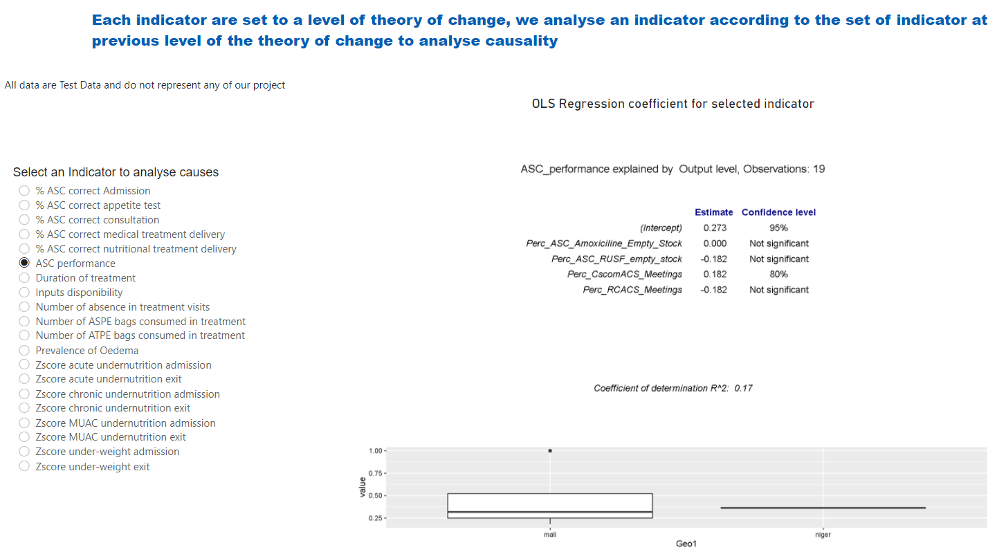
In this pbix File, we construct an analysis of Theory of change and create a R visual that gather a regression analysis and a Boxplot visual.

Theory of change is a theoritical relation between indicators:
Gestion -> Output -> Outcome -> Impact
How we do -> What we do -> Why we do -> General Objective
- Mark as New
- Bookmark
- Subscribe
- Mute
- Subscribe to RSS Feed
- Permalink
- Report Inappropriate Content
02-05-2025
02:30 AM
UPDATE 02/2025:
library(tidyr)
library(ggplot2)
library(stringr)
library(gridExtra)
library(gtable)
library(grid)
library(ggpubr)
names(dataset)[names(dataset)=="DB_Standard_Indicators/INDICATOR_value"]<-"value"
names(dataset)[names(dataset)=="DB_Standard_Indicators/INDICATOR_level"]<-"level"
names(dataset)[names(dataset)=="DB_Standard_Indicators/modality_intervention"]<-"modality"
names(dataset)[names(dataset)=="DB_Standard_Indicators/INDICATOR_code"]<-"code"
names(dataset)[names(dataset)=="_id"]<-"id"
names(dataset)[names(dataset)=="Selected_Y"]<-"Y"
names(dataset)[names(dataset)=="DB_Standard_Indicators/INDICATOR_analisis_unit"]<-"analisis_unit"
names(dataset)[names(dataset)=="DB_Standard_Indicators/INDICATOR_Geo1"]<-"Geo1"
names(dataset)[names(dataset)=="DB_Standard_Indicators/INDICATOR_Geo2"]<-"Geo2"
names(dataset)[names(dataset)=="DB_Standard_Indicators/INDICATOR_Geo3"]<-"Geo3"
names(dataset)[names(dataset)=="DB_Standard_Indicators/INDICATOR_Geo4"]<-"Geo4"
dataset$Y<-str_replace_all(dataset$Y, "%", "Perc")
dataset$code<-str_replace_all(dataset$code, "%", "Perc")
dataset$Y<-str_replace_all(dataset$Y, "[[:punct:]]", "")
dataset$code<-str_replace_all(dataset$code, "[[:punct:]]", "")
dataset$Y<-str_replace_all(dataset$Y, " ", "_")
dataset$code<-str_replace_all(dataset$code, " ", "_")
Info_Y<-head(subset(dataset,dataset$code==as.character(Y),select=c( level, modality, code,analisis_unit)),1)
DependentVar<-as.character(Info_Y$code[1])
Selected_Level_Analisis=(Info_Y[1,1])
Analised_by_Level=ifelse(Selected_Level_Analisis=="Impact","Outcome",ifelse(Selected_Level_Analisis=="Outcome","Output","Gestion"))
# Analyzing the outcome selected by the output of the same level
df_Y<-subset(dataset,dataset$code==as.character(Y),select=c( value, Y,Geo4,id))
df_Y$Y<-"Y"
df_Y_BXPL<-subset(dataset,dataset$code==as.character(Y),select=c( value, Y,Geo1,Geo2,Geo3,Geo4,id))
bxplot<-ggplot(df_Y_BXPL, aes(x=Geo1, y=value))+geom_boxplot()+ stat_compare_means(method = "t.test")
Spreaddf_Y<-spread(df_Y,Y,value)
df_X<-subset(dataset,level==Analised_by_Level,select=c( value, level, modality, code,id,analisis_unit,Geo1,Geo2,Geo3,Geo4))
df_X<-subset(df_X,analisis_unit==as.character(Info_Y$analisis_unit[1]),select=c( value, level, modality, code,id,analisis_unit,Geo1,Geo2,Geo3,Geo4))
Spreaddf_X<-spread(df_X,code,value)
final<-merge(Spreaddf_Y,Spreaddf_X,by="Geo4")
final<-subset(final,select=-c(Geo4,id.x,level,modality,id.y,analisis_unit,Geo1,Geo2,Geo3))
model<-lm(Y~.,data=final)
resumen<-summary(model)
r2<-round(resumen$r.squared,2)
coefficient<-round(resumen$coefficients,3)
coefficient<-subset(coefficient,select=c("Estimate","Pr(>|t|)"))
colnames(coefficient)[1]<-"Estimate"
colnames(coefficient)[2]<-"Significance"
coefficient <- transform(coefficient, Significance = ifelse(Significance < 0.05, "95%", ifelse(Significance < 0.1, "90%", ifelse(Significance < 0.15, "85%", ifelse(Significance < 0.20, "80%", "Not significant")))))
colnames(coefficient)[2]<-"Confidence level"
Num_Obs<-length(fitted(model))
title <- textGrob(paste(DependentVar, "explained by ",Analised_by_Level,"level, Observations:" , Num_Obs) ,gp=gpar(fontsize=14))
footnote <- textGrob(paste("Coefficient of determination R^2: ",r2), x=0.5, hjust=0.5,gp=gpar( fontface="italic"))
padding<- textGrob( " " ,gp=gpar(fontsize=14))
mytheme<-ttheme_minimal(colhead=list(fg_params=list(col="navyblue")))
table <- tableGrob(coefficient,theme=mytheme)
grid.arrange(title,arrangeGrob(table,ncol=1,nrow=2),arrangeGrob(footnote,ncol=1,nrow=1),arrangeGrob(bxplot,ncol=1,nrow=1),ncol=1)
- Mark as New
- Bookmark
- Subscribe
- Mute
- Subscribe to RSS Feed
- Permalink
- Report Inappropriate Content
07-15-2024
09:00 AM
UPDATE 'base2grob' is no longer available
Here is an adapted version with ggplot2.
I've also performed a t-test that check whether there is sufficient observations or not.
Here is the visual code:
library(tidyr)
library(ggplot2)
library(stringr)
library(gridExtra)
library(gtable)
library(grid)
library(ggpubr)
names(dataset)[names(dataset)=="DB_Standard_Indicators/INDICATOR_value"]<-"value"
names(dataset)[names(dataset)=="DB_Standard_Indicators/INDICATOR_level"]<-"level"
names(dataset)[names(dataset)=="DB_Standard_Indicators/modality_intervention"]<-"modality"
names(dataset)[names(dataset)=="DB_Standard_Indicators/INDICATOR_code"]<-"code"
names(dataset)[names(dataset)=="_id"]<-"id"
names(dataset)[names(dataset)=="Selected_Y"]<-"Y"
names(dataset)[names(dataset)=="DB_Standard_Indicators/INDICATOR_analisis_unit"]<-"analisis_unit"
names(dataset)[names(dataset)=="DB_Standard_Indicators/INDICATOR_Geo1"]<-"Geo1"
names(dataset)[names(dataset)=="DB_Standard_Indicators/INDICATOR_Geo2"]<-"Geo2"
names(dataset)[names(dataset)=="DB_Standard_Indicators/INDICATOR_Geo3"]<-"Geo3"
names(dataset)[names(dataset)=="DB_Standard_Indicators/INDICATOR_Geo4"]<-"Geo4"
dataset$Y<-str_replace_all(dataset$Y, "%", "Perc")
dataset$code<-str_replace_all(dataset$code, "%", "Perc")
dataset$Y<-str_replace_all(dataset$Y, "[[:punct:]]", "")
dataset$code<-str_replace_all(dataset$code, "[[:punct:]]", "")
dataset$Y<-str_replace_all(dataset$Y, " ", "_")
dataset$code<-str_replace_all(dataset$code, " ", "_")
Info_Y<-head(subset(dataset,dataset$code==as.character(Y),select=c(level, modality, code,analisis_unit)),1)
DependentVar<-as.character(Info_Y$code[1])
Selected_Level_Analisis=(Info_Y[1,1])
Analised_by_Level=ifelse(Selected_Level_Analisis=="Impact","Outcome",ifelse(Selected_Level_Analisis=="Outcome","Output","Gestion"))
# empezamos con analyzar el outcome seleccionado por los output del mismo nivel de analisis
df_Y<-subset(dataset,dataset$code==as.character(Y),select=c(value, Y,Geo4,id))
df_Y$Y<-"Y"
df_Y_BXPL<-subset(dataset,dataset$code==as.character(Y),select=c(value, Y,Geo1,Geo2,Geo3,Geo4,id))
# Try to perform t-test and handle errors due to insufficient observations
ttest_result <- tryCatch(t.test(value ~ Geo1, data = df_Y_BXPL), error = function(e) NULL)
if (is.null(ttest_result)) {
p_value <- NA
significance_sentence <- "There are not sufficient observations to perform the t-test."
} else {
p_value <- ttest_result$p.value
significance_sentence <- ifelse(p_value < 0.05, "There is a significant difference among the categories (p < 0.05).", "There is no significant difference among the categories (p >= 0.05).")
}
bxplot <- ggplot(df_Y_BXPL, aes(x=Geo1, y=value)) +
geom_boxplot() +
stat_compare_means(method = "t.test", label = "p.format") +
ggtitle(significance_sentence)
Spreaddf_Y<-spread(df_Y,Y,value)
df_X<-subset(dataset,level==Analised_by_Level,select=c(value, level, modality, code,id,analisis_unit,Geo1,Geo2,Geo3,Geo4))
df_X<-subset(df_X,analisis_unit==as.character(Info_Y$analisis_unit[1]),select=c(value, level, modality, code,id,analisis_unit,Geo1,Geo2,Geo3,Geo4))
Spreaddf_X<-spread(df_X,code,value)
final<-merge(Spreaddf_Y,Spreaddf_X,by="Geo4")
final<-subset(final,select=-c(Geo4,id.x,level,modality,id.y,analisis_unit,Geo1,Geo2,Geo3))
model<-lm(Y~.,data=final)
resumen<-summary(model)
r2<-round(resumen$r.squared,2)
coefficient<-round(resumen$coefficients,3)
coefficient<-subset(coefficient,select=c("Estimate","Pr(>|t|)"))
colnames(coefficient)[1]<-"Estimate"
colnames(coefficient)[2]<-"Significance"
coefficient <- transform(coefficient, Significance = ifelse(Significance < 0.05, "95%", ifelse(Significance < 0.1, "90%", ifelse(Significance < 0.15, "85%", ifelse(Significance < 0.20, "80%", "Not significant")))))
colnames(coefficient)[2]<-"Confidence level"
Num_Obs<-length(fitted(model))
# Create title, footnote, and table using ggplot2
title_plot <- ggplot() +
annotate("text", x = 1, y = 1, label = paste(DependentVar, "explained by ", Analised_by_Level, "level, Observations:", Num_Obs), size = 6) +
theme_void()
footnote_plot <- ggplot() +
annotate("text", x = 1, y = 1, label = paste("Coefficient of determination R^2: ", r2), size = 5, fontface = "italic") +
theme_void()
table_plot <- ggplot() +
theme_void() +
annotation_custom(tableGrob(coefficient, theme = ttheme_minimal(colhead = list(fg_params = list(col = "navyblue")))), xmin = -Inf, xmax = Inf, ymin = -Inf, ymax = Inf)
# Arrange the plots using gridExtra
final_plot <- grid.arrange(
title_plot,
table_plot,
footnote_plot,
bxplot,
ncol = 1,
heights = c(0.1, 0.4, 0.1, 0.4)
)
# Print the final plot
print(final_plot)